Nonlinear System with Cross-Coupling Between Components

This example shows how to solve a nonlinear PDE system of two equations with cross-coupling between the two components. The system is a Schnakenberg system

$$\begin{array}{l}\frac{\partial {\mathit{u}}_1}{\partial \mathit{t}}-{\mathit{D}}_1\Delta {\mathit{u}}_1=\kappa \left(\mathit{a}-{\mathit{u}}_1+{{\mathit{u}}_1}^2{\mathit{u}}_2\right)\\ \frac{\partial {\mathit{u}}_2}{\partial \mathit{t}}-{\mathit{D}}_2\Delta {\mathit{u}}_2=\kappa \left(\mathit{b}-{{\mathit{u}}_1}^2{\mathit{u}}_2\right)\end{array}$$

with the steady-state solution ${\mathit{u}}_{1\mathit{S}}=\mathit{a}+\mathit{b}$ and ${\mathit{u}}_{2\mathit{S}}=\frac{\mathit{b}}{{\left(\mathit{a}+\mathit{b}\right)}^2}$. The initial conditions are a small perturbation of the steady-state solution.

Solution for First Time Span

First, create a PDE model for a system of two equations.

model = createpde(2);

Create a cubic geometry and assign it to the model.

gm = multicuboid(1,1,1);
model.Geometry = gm;

Generate the mesh using the linear geometric order to save memory.

generateMesh(model,GeometricOrder="linear");

Define the parameters of the system.

D1 = 0.05;
D2 = 1;
kappa = 100;
a = 0.2;
b = 0.8;

Based on these parameters, specify the PDE coefficients in the toolbox format.

d = [1;1];
c = [D1;D2];
f = @(region,state) [kappa*(a - state.u(1,:) + ...
                            state.u(1,:).^2.*state.u(2,:));
                     kappa*(b - state.u(1,:).^2.*state.u(2,:))
                    ];
specifyCoefficients(model,m=0,d=d,c=c,a=0,f=f);

Set the initial conditions. The first component is a small perturbation of the steady-state solution ${\mathit{u}}_{1\mathit{S}}=\mathit{a}+\mathit{b}$. The second component is the steady-state solution ${\mathit{u}}_{2\mathit{S}}=\frac{\mathit{b}}{{\left(\mathit{a}+\mathit{b}\right)}^2}$.

icFcn = @(region) [a + b + 10^(-3)*exp(-100*((region.x - 1/3).^2 ...
                   + (region.y - 1/2).^2)); ...
                   (b/(a + b)^2)*ones(size(region.x))];

setInitialConditions(model,icFcn);

Solve the system for times 0 through 2 seconds.

tlist = linspace(0,2,10);
results = solvepde(model,tlist);

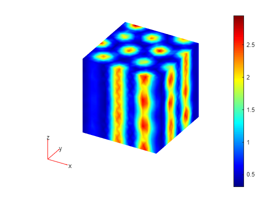
Plot the first component of the solution at the last time step.

pdeplot3D(model,ColorMapData=results.NodalSolution(:,1,end));

Initial Condition for Second Time Span Based on Previous Solution

Now, resume the analysis and solve the problem for times from 2 to 5 seconds. Reduce the magnitude of the previously obtained solution for time 2 seconds to 10% of the original value.

u2 = results.NodalSolution(:,:,end);
newResults = createPDEResults(model,u2(:)*0.1);

Use newResults as the initial condition for further analysis.

setInitialConditions(model,newResults);

Solve the system for times 2 through 5 seconds.

tlist = linspace(2,5,10);
results25 = solvepde(model,tlist);

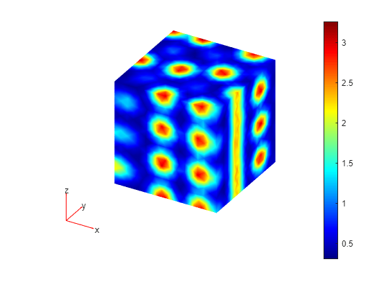
Plot the first component of the solution at the last time step.

figure
pdeplot3D(model,ColorMapData=results25.NodalSolution(:,1,end));

Alternatively, you can write a function that uses the results returned by the solver and computes the initial conditions based on the results of the previous analysis.

function newU0 = computeNewIC(resultsObject)
newU0 = 0.1*resultsObject.NodalSolution(:,:,end).';
end

Remove the previous initial conditions.

delete(model.InitialConditions);

Set the initial conditions using the function NewIC.

NewIC = @(location) computeNewIC(results);
setInitialConditions(model,NewIC)

ans = 
  GeometricInitialConditions with properties:

           RegionType: 'cell'
             RegionID: 1
         InitialValue: @(location)computeNewIC(results)
    InitialDerivative: []

Solve the system for times 2 through 5 seconds.

results25f = solvepde(model,tlist);

Plot the first component of the solution at the last time step.

figure
pdeplot3D(model,ColorMapData=results25f.NodalSolution(:,1,end));