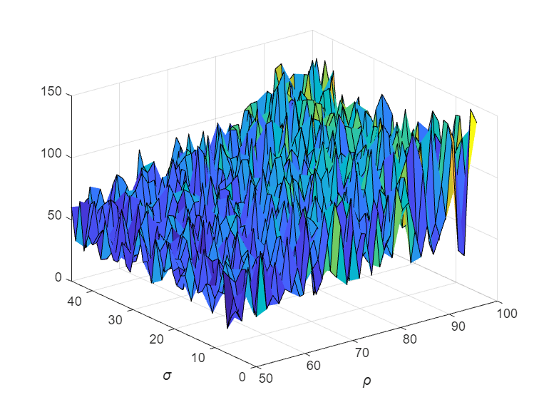
Plot During Parameter Sweep with parfeval

This example shows how to perform a parallel parameter sweep with parfeval and send results back during computations with a DataQueue object.

parfeval does not block MATLAB, so you can continue working while computations take place.

The example performs a parameter sweep on the Lorenz system of ordinary differential equations, on the parameters $\sigma$ and $\rho$, and shows the chaotic nature of this system.

$$\begin{array}{l}\frac{\mathrm{d}}{\mathrm{d}\mathit{t}}\mathit{x}=\sigma \left(\mathit{y}-\mathit{z}\right)\\ \frac{\mathrm{d}}{\mathrm{d}\mathit{t}}\mathit{y}=\mathit{x}\left(\rho -\mathit{z}\right)-\mathit{y}\\ \frac{\mathrm{d}}{\mathrm{d}\mathit{t}}\mathit{z}=\mathit{xy}-\beta \mathit{x}\end{array}$$

Set Up Parallel Environment

Create a pool of parallel of thread workers by using the parpool function.

parpool("Threads");

Starting parallel pool (parpool) using the 'Threads' profile ...
Connected to parallel pool with 6 workers.

Create Parameter Grid

Define the range of parameters that you want to explore in the parameter sweep.

gridSize = 40;
sigma = linspace(5,45,gridSize);
rho = linspace(50,100,gridSize);
beta = 8/3;

Create a 2-D grid of parameters by using the meshgrid function.

[rho,sigma] = meshgrid(rho,sigma);

Perform Parallel Parameter Sweep

After you define the parameters, you can perform the parallel parameter sweep.

To visualize the interim results of the parameter sweep, create a surface plot. Note that initializing the Z component of the surface with NaN creates an empty plot.

figure;
surface = surf(rho,sigma,NaN(size(sigma)));
xlabel('\rho','Interpreter','Tex')
ylabel('\sigma','Interpreter','Tex')

To send interim data from the workers, create a DataQueue object. Set up a function that updates the surface plot each time a worker sends data by using the afterEach function. The updatePlot function is a supporting function defined at the end of the example.

Q = parallel.pool.DataQueue;
afterEach(Q,@(data) updatePlot(surface,data));

parfeval works more efficiently when you distribute the workload. To distribute the workload, group the parameters to explore into partitions. For this example, split into uniform partitions of size step by using the colon operator (:). The resulting array partitions contains the boundaries of the partitions. Note that you must add the end point of the last partition.

step = 100;
partitions = [1:step:numel(sigma),numel(sigma)+1]

partitions = 1×17

           1         101         201         301         401         501         601         701         801         901        1001        1101        1201        1301        1401        1501        1601

For best performance, try to split into partitions that are:

• Large enough that the computation time is large compared to the overhead of scheduling the partition.

• Small enough that there are enough partitions to keep all workers busy.

To represent function executions on parallel workers and hold their results, use future objects.

f(1:numel(partitions)-1) = parallel.FevalFuture;

Offload computations to parallel workers by using the parfeval function. parameterSweep is a helper function defined at the end of this script that solves the Lorenz system on a partition of the parameters to explore. It has one output argument, so you must specify 1 as the number of outputs in parfeval.

for ii = 1:numel(partitions)-1
    f(ii) = parfeval(@parameterSweep,1,partitions(ii),partitions(ii+1),sigma,rho,beta,Q);
end

parfeval does not block MATLAB, so you can continue working while computations take place. The workers compute in parallel and send intermediate results through the DataQueue as soon as they become available.

If you want to block MATLAB until parfeval completes, use the wait function on the future objects. Using the wait function is useful when subsequent code depends on the completion of parfeval.

wait(f);

After parfeval finishes the computations, wait finishes and you can execute more code. For example, plot a selection of the Lorenz system solutions. Use the fetchOutputs function to retrieve the results stored in the future objects.

results = fetchOutputs(f);
idxs = randperm(numel(results),4);
figure
for n = 1:numel(idxs)
    nexttile
    a = results{idxs(n)};
    plot3(a(:,1),a(:,2),a(:,3))
    grid on
    xlabel("x")
    ylabel("y")
    zlabel("z")
    title("Lorenz System Solution", ...
        "\rho = "+ num2str(rho(idxs(n)),'%5.2f') + " \sigma = "+ num2str(sigma(idxs(n)),'%5.2f'),Interpreter="tex")
end

If your parameter sweep needs more computational resources and you have access to a cluster, you can scale up your parfeval computations. For more information, see Scale Up from Desktop to Cluster.

Define Helper Functions

Define a helper function that solves the Lorenz system on a partition of the parameters to explore. Send intermediate results to the MATLAB client by using the send function on the DataQueue object.

function results = parameterSweep(first,last,sigma,rho,beta,Q)
    results = cell(last-first,1);
    for ii = first:last-1
        lorenzSystem = @(t,a) [sigma(ii)*(a(2) - a(1)); a(1)*(rho(ii) - a(3)) - a(2); a(1)*a(2) - beta*a(3)];
        [t,a] = ode45(lorenzSystem,[0 100],[1 1 1]);
        send(Q,[ii,a(end,3)]);
        results{ii-first+1} = a;
    end
end

Define another helper function that updates the surface plot when new data arrives.

function updatePlot(surface,data)
    surface.ZData(data(1)) = data(2);
    drawnow('limitrate');
end