Maximize Long-Term Investments Using Linear Programming: Problem-Based
This example shows how to use the problem-based approach to solve an investment problem with deterministic returns over a fixed number of years T. The problem is to allocate your money over available investments to maximize your final wealth. For the solver-based approach, see Maximize Long-Term Investments Using Linear Programming: Solver-Based.
Problem Formulation
Suppose that you have an initial amount of money Capital_0 to invest over a time period of T years in N zero-coupon bonds. Each bond pays a fixed interest rate, compounds the investment each year, and pays the principal plus compounded interest at the end of a maturity period. The objective is to maximize the total amount of money returned after T years.
You can include a constraint that no single investment is more than a certain fraction of your total capital at the time of the investment.
This example shows the problem setup on a small case first, and then formulates the general case.
You can model this as a linear programming problem. Therefore, to optimize your wealth, formulate the problem using the optimization problem approach.
Introductory Example
Start with a small example:
The starting amount to invest
Capital_0is $1000.The time period
Tis 5 years.The number of bonds
Nis 4.To model uninvested money, have one option B0 available every year that has a maturity period of 1 year and an interest rate of 0%.
Bond 1, denoted by B1, can be purchased in year 1, has a maturity period of 4 years, and an interest rate of 2%.
Bond 2, denoted by B2, can be purchased in year 5, has a maturity period of 1 year, and an interest rate of 4%.
Bond 3, denoted by B3, can be purchased in year 2, has a maturity period of 4 years, and an interest rate of 6%.
Bond 4, denoted by B4, can be purchased in year 2, has a maturity period of 3 years, and an interest rate of 6%.
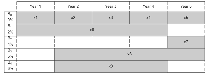
By splitting up the first option B0 into 5 bonds with maturity period of 1 year and interest rate of 0%, this problem can be equivalently modeled as having a total of 9 available bonds, such that for k=1..9
Entry
kof vectorPurchaseYearsrepresents the beginning of the year that bondkis available for purchase.Entry
kof vectorMaturityrepresents the maturity period of bondk.Entry
kof vectorMaturityYearsrepresents the end of the year that bondkis available for sale.Entry
kof vectorInterestRatesrepresents the percentage interest rate of bondk.
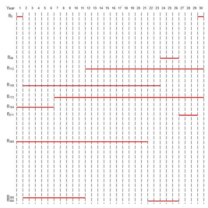
Visualize this problem by horizontal bars that represent the available purchase times and durations for each bond.
% Time period in years
T = 5;
% Number of bonds
N = 4;
% Initial amount of money
Capital_0 = 1000;
% Total number of buying opportunities
nPtotal = N+T;
% Purchase times
PurchaseYears = [1;2;3;4;5;1;5;2;2];
% Bond durations
Maturity = [1;1;1;1;1;4;1;4;3];
% Bond sale times
MaturityYears = PurchaseYears + Maturity - 1;
% Interest rates in percent
InterestRates = [0;0;0;0;0;2;4;6;6];
% Return after one year of interest
rt = 1 + InterestRates/100;

plotInvestments(N,PurchaseYears,Maturity,InterestRates)
Decision Variables
Represent your decision variables by a vector x, where x(k) is the dollar amount of investment in bond k, for k = 1,...,9. Upon maturity, the payout for investment x(k) is
Define and define as the total return of bond k:
x = optimvar("x",nPtotal,LowerBound=0);
% Total returns
r = rt.^Maturity;
Objective Function
The goal is to choose investments to maximize the amount of money collected at the end of year T. From the plot, you see that investments are collected at various intermediate years and reinvested. At the end of year T, the money returned from investments 5, 7, and 8 can be collected and represents your final wealth:
Create an optimization problem for maximization, and include the objective function.
interestprob = optimproblem(ObjectiveSense="maximize");
interestprob.Objective = x(5)*r(5) + x(7)*r(7) + x(8)*r(8);
Linear Constraints: Invest No More Than You Have
Every year, you have a certain amount of money available to purchase bonds. Starting with year 1, you can invest the initial capital in the purchase options and , so:
Then for the following years, you collect the returns from maturing bonds, and reinvest them in new available bonds to obtain the system of equations:
investconstr = optimconstr(T,1);
investconstr(1) = x(1) + x(6) == Capital_0;
investconstr(2) = x(2) + x(8) + x(9) == r(1)*x(1);
investconstr(3) = x(3) == r(2)*x(2);
investconstr(4) = x(4) == r(3)*x(3);
investconstr(5) = x(5) + x(7) == r(4)*x(4) + r(6)*x(6) + r(9)*x(9);
interestprob.Constraints.investconstr = investconstr;
Bound Constraints: No Borrowing
Because each amount invested must be positive, each entry in the solution vector must be positive. Include this constraint by setting a lower bound on the solution vector . There is no explicit upper bound on the solution vector.
x.LowerBound = 0;
Solve the Problem
Solve this problem with no constraints on the amount you can invest in a bond. The interior-point algorithm can be used to solve this type of linear programming problem.
options = optimoptions("linprog",Algorithm="interior-point");
[sol,fval,exitflag] = solve(interestprob,Options=options)
Solving problem using linprog.

Solution found during presolve.
sol = struct with fields:
    x: [9×1 double]
fval =
1.2625e+03
exitflag =
    OptimalSolution
Visualize the Solution
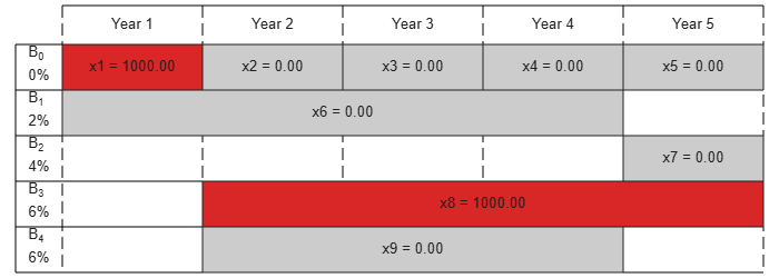
The exit flag indicates that the solver found an optimal solution. The value fval, returned as the second output argument, corresponds to the final wealth. Look at the final sum of investments, and the investment allocation over time.
fprintf("After %d years, the return for the initial $%g is $%g \n",...
    T,Capital_0,fval);
After 5 years, the return for the initial $1000 is $1262.48
plotInvestments(N,PurchaseYears,Maturity,InterestRates,sol.x)
Optimal Investment with Limited Holdings
To diversify your investments, you can choose to limit the amount invested in any one bond to a certain percentage Pmax of the total capital that year (including the returns for bonds that are currently in their maturity period). You obtain the following system of inequalities:
% Maximum percentage to invest in any bond
Pmax = 0.6;
constrlimit = optimconstr(nPtotal,1);
constrlimit(1) = x(1) <= Pmax*Capital_0;
constrlimit(2) = x(2) <= Pmax*(rt(1)*x(1) + rt(6)*x(6));
constrlimit(3) = x(3) <= Pmax*(rt(2)*x(2) + rt(6)^2*x(6) + rt(8)*x(8) + rt(9)*x(9));
constrlimit(4) = x(4) <= Pmax*(rt(3)*x(3) + rt(6)^3*x(6) + rt(8)^2*x(8) + rt(9)^2*x(9));
constrlimit(5) = x(5) <= Pmax*(rt(4)*x(4) + rt(6)^4*x(6) + rt(8)^3*x(8) + rt(9)^3*x(9));
constrlimit(6) = x(6) <= Pmax*Capital_0;
constrlimit(7) = x(7) <= Pmax*(rt(4)*x(4) + rt(6)^4*x(6) + rt(8)^3*x(8) + rt(9)^3*x(9));
constrlimit(8) = x(8) <= Pmax*(rt(1)*x(1) + rt(6)*x(6));
constrlimit(9) = x(9) <= Pmax*(rt(1)*x(1) + rt(6)*x(6));
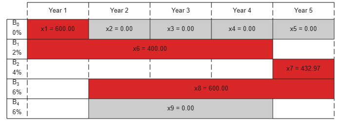
interestprob.Constraints.constrlimit = constrlimit;Solve the problem by investing no more than 60% in any one asset. Plot the resulting purchases. Notice that your final wealth is less than the investment without this constraint.
[sol,fval] = solve(interestprob,Options=options);
Solving problem using linprog.

Minimum found that satisfies the constraints.

Optimization completed because the objective function is non-decreasing in feasible directions, to within the function tolerance, and constraints are satisfied to within the constraint tolerance.
fprintf("After %d years, the return for the initial $%g is $%g \n",...
    T,Capital_0,fval);
After 5 years, the return for the initial $1000 is $1207.78
plotInvestments(N,PurchaseYears,Maturity,InterestRates,sol.x)
Model of Arbitrary Size
Create a model for a general version of the problem. Illustrate it using T = 30 years and 400 randomly generated bonds with interest rates from 1 to 6%. This setup results in a linear programming problem with 430 decision variables.
% For reproducibility
rng default
% Initial amount of money
Capital_0 = 1000;
% Time period in years
T = 30;
% Number of bonds
N = 400;
% Total number of buying opportunities
nPtotal = N + T;
% Generate random maturity durations
Maturity = randi([1 T-1],nPtotal,1);
% Bond 1 has a maturity period of 1 year
Maturity(1:T) = 1;
% Generate random yearly interest rate for each bond
InterestRates = randi(6,nPtotal,1);
% Bond 1 has an interest rate of 0 (not invested)
InterestRates(1:T) = 0;
% Return after one year of interest
rt = 1 + InterestRates/100;
% Compute the return at the end of the maturity period for each bond:
r = rt.^Maturity;

% Generate random purchase years for each option
PurchaseYears = zeros(nPtotal,1);
% Bond 1 is available for purchase every year
PurchaseYears(1:T)=1:T;
for i=1:N
    % Generate a random year for the bond to mature before the end of
    % the T year period
    PurchaseYears(i+T) = randi([1 T-Maturity(i+T)+1]);
end

% Compute the years where each bond reaches maturity at the end of the year
MaturityYears = PurchaseYears + Maturity - 1;
Compute the times when bonds can be bought or sold. The buyindex matrix holds the potential purchase times, and the sellindex matrix holds the potential sales times for each bond.
buyindex = false(nPtotal,T); % allocate nPtotal-by-T matrix
for ii = 1:T
    buyindex(:,ii) = PurchaseYears == ii;
end
sellindex = false(nPtotal,T);
for ii = 1:T
    sellindex(:,ii) = MaturityYears == ii;
end
Set up the optimization variables corresponding to the bonds.
x = optimvar("x",nPtotal,1,LowerBound=0);Create the optimization problem and objective function.
interestprob = optimproblem(ObjectiveSense="maximize");
interestprob.Objective = sum(x(sellindex(:,T)).*r(sellindex(:,T)));
For convenience, create a temporary array xBuy, whose columns represent the bonds we can buy at each time period.
xBuy = repmat(x,1,T).*double(buyindex);
Similarly, create a temporary array xSell, whose columns represent the bonds we can sell at each time period.
xSell = repmat(x,1,T).*double(sellindex);
The return generated for selling these bounds is
xReturnFromSell = xSell.*repmat(r,1,T);
Create the constraint that the amount you invest in each time period is the amount that you sold in the previous time period.
interestprob.Constraints.InitialInvest = sum(xBuy(:,1)) == Capital_0;
interestprob.Constraints.InvestConstraint = sum(xBuy(:,2:T),1) == sum(xReturnFromSell(:,1:T-1),1);
Solution with No Holding Limit
Solve the problem.
tic
[sol,fval,exitflag] = solve(interestprob,Options=options);
Solving problem using linprog.

Solution found during presolve.
toc
Elapsed time is 0.086600 seconds.
How well did the investments do?
fprintf("After %d years, the return for the initial $%g is $%g \n",...
    T,Capital_0,fval);
After 30 years, the return for the initial $1000 is $5167.58
Solution with Limited Holdings
To create constraints that limit the fraction of investments in each asset, set up a matrix that keeps track of the active bonds at each time. To express the constraint that each investment must be less than Pmax times the total value, set up a matrix that keeps track of the value of each investment at each time. For this larger problem, set the maximum fraction that can be held to 0.4.
Pmax = 0.4;
Create an active matrix corresponding to times when a bond can be held, and a cactive matrix that holds the cumulative duration of each active bond. So the value of bond j at time t is x(j)*(rt^cactive).
active = double(buyindex | sellindex);
for ii = 1:T
    active(:,ii) = double((ii >= PurchaseYears) & (ii <= MaturityYears));
end
cactive = cumsum(active,2);
cactive = cactive.*active;
Create the matrix whose entry (j,p) represents the value of bond j at time period p:
bondValue = repmat(x, 1, T).*active.*(rt.^(cactive));
Determine the total value of the investments at each time interval so you can impose the constraint on limited holdings. mvalue is the money invested in all the bonds at the end of each time period, an nPtotal-by-T matrix.moneyavailable is the sum over the bonds of the money invested at the beginning of the time period, meaning the value of the portfolio at each time.
constrlimit = optimconstr(nPtotal,T);
constrlimit(:,1) = xBuy(:,1) <= Pmax*Capital_0;
constrlimit(:,2:T) = xBuy(:,2:T)  <= repmat(Pmax*sum(bondValue(:,1:T-1),1), nPtotal, 1).*double(buyindex(:,2:T));
interestprob.Constraints.constrlimit = constrlimit;
Solve the problem with limited holdings.
tic
[sol,fval,exitflag] = solve(interestprob,Options=options);
Solving problem using linprog.

Minimum found that satisfies the constraints.

Optimization completed because the objective function is non-decreasing in feasible directions, to within the function tolerance, and constraints are satisfied to within the constraint tolerance.
toc
Elapsed time is 1.639808 seconds.
fprintf("After %d years, the return for the initial $%g is $%g \n",...
    T,Capital_0,fval);
After 30 years, the return for the initial $1000 is $5095.26
To speed up the solver, try the dual-simplex algorithm.
options = optimoptions("linprog",Algorithm="dual-simplex");
tic
[sol,fval,exitflag] = solve(interestprob,Options=options);
Solving problem using linprog.

Optimal solution found.
toc
Elapsed time is 0.139493 seconds.
fprintf("After %d years, the return for the initial $%g is $%g \n",...
    T,Capital_0,fval);
After 30 years, the return for the initial $1000 is $5095.26
In this case, the dual-simplex algorithm took less time to obtain the same solution.
Qualitative Result Analysis
To get a feel for the solution, compare it to the amount fmax that you would get if you could invest all of your starting money in one bond with a 6% interest rate (the maximum interest rate) over the full 30 year period. You can also compute the equivalent interest rate corresponding to your final wealth.
% Maximum amount
fmax = Capital_0*(1+6/100)^T;
% Ratio (in percent)
rat = fval/fmax*100;
% Equivalent interest rate (in percent)
rsol = ((fval/Capital_0)^(1/T)-1)*100;

fprintf(['The amount collected is %g%% of the maximum amount $%g '...
    'that you would obtain from investing in one bond.\n'...
    'Your final wealth corresponds to a %g%% interest rate over the %d year '...
    'period.\n'], rat, fmax, rsol, T)
The amount collected is 88.7137% of the maximum amount $5743.49 that you would obtain from investing in one bond.
Your final wealth corresponds to a 5.57771% interest rate over the 30 year period.
plotInvestments(N,PurchaseYears,Maturity,InterestRates,sol.x,false)