Fit an Ordinary Differential Equation (ODE)
This example shows how to fit parameters of an ODE to data in two ways. The first shows a straightforward fit of a constant-speed circular path to a portion of a solution of the Lorenz system, a famous ODE with sensitive dependence on initial parameters. The second shows how to modify the parameters of the Lorenz system to fit a constant-speed circular path. You can use the appropriate approach for your application as a model for fitting a differential equation to data.
Lorenz System: Definition and Numerical Solution
The Lorenz system is a system of ordinary differential equations (see Lorenz system). For real constants , the system is
Lorenz's values of the parameters for a sensitive system are . Start the system from [x(0),y(0),z(0)] = [10,20,10] and view the evolution of the system from time 0 through 100.
sigma = 10;
beta = 8/3;
rho = 28;
f = @(t,a) [-sigma*a(1) + sigma*a(2); rho*a(1) - a(2) - a(1)*a(3); -beta*a(3) + a(1)*a(2)];
xt0 = [10,20,10];
[tspan,a] = ode45(f,[0 100],xt0);     % Runge-Kutta 4th/5th order ODE solver
figure
plot3(a(:,1),a(:,2),a(:,3))
view([-10.0 -2.0])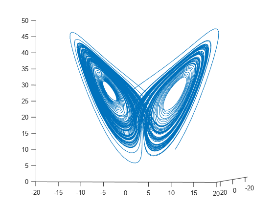
The evolution is quite complicated. But over a small time interval, it looks somewhat like uniform circular motion. Plot the solution over the time interval [0,1/10].
[tspan,a] = ode45(f,[0 1/10],xt0);     % Runge-Kutta 4th/5th order ODE solver
figure
plot3(a(:,1),a(:,2),a(:,3))
view([-30 -70])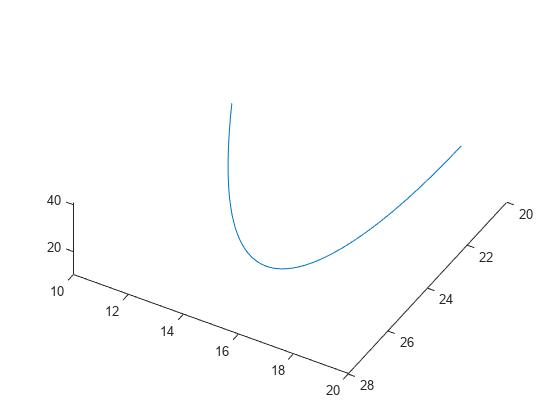
Fit a Circular Path to the ODE Solution
The equations of a circular path have several parameters:
Angle of the path from the x-y plane
Angle of the plane from a tilt along the x-axis
Radius R
Speed V
Shift t0 from time 0
3-D shift in space delta
In terms of these parameters, determine the position of the circular path for times xdata.
function f = fitlorenzfn(x,xdata)

theta = x(1:2);
R = x(3);
V = x(4);
t0 = x(5);
delta = x(6:8);
f = zeros(length(xdata),3);
f(:,3) = R*sin(theta(1))*sin(V*(xdata - t0)) + delta(3);
f(:,1) = R*cos(V*(xdata - t0))*cos(theta(2)) ...
    - R*sin(V*(xdata - t0))*cos(theta(1))*sin(theta(2)) + delta(1);
f(:,2) = R*sin(V*(xdata - t0))*cos(theta(1))*cos(theta(2)) ...
    - R*cos(V*(xdata - t0))*sin(theta(2)) + delta(2);
end
To find the best-fitting circular path to the Lorenz system at times given in the ODE solution, use lsqcurvefit. In order to keep the parameters in reasonable limits, put bounds on the various parameters.
lb = [-pi/2,-pi,5,-15,-pi,-40,-40,-40];
ub = [pi/2,pi,60,15,pi,40,40,40];
theta0 = [0;0];
R0 = 20;
V0 = 1;
t0 = 0;
delta0 = zeros(3,1);
x0 = [theta0;R0;V0;t0;delta0];
[xbest,resnorm,residual] = lsqcurvefit(@fitlorenzfn,x0,tspan,a,lb,ub);
Local minimum possible.

lsqcurvefit stopped because the final change in the sum of squares relative to
its initial value is less than the value of the function tolerance.

<stopping criteria details>
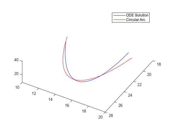
Plot the best-fitting circular points at the times from the ODE solution together with the solution of the Lorenz system.
soln = a + residual;
hold on
plot3(soln(:,1),soln(:,2),soln(:,3),"r")
legend("ODE Solution","Circular Arc")
hold off
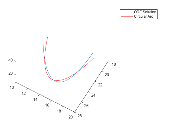
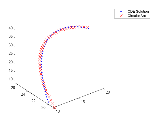
figure
plot3(a(:,1),a(:,2),a(:,3),"b.",MarkerSize=10)
hold on
plot3(soln(:,1),soln(:,2),soln(:,3),"rx",MarkerSize=10)
legend("ODE Solution","Circular Arc")
hold off
Fit the ODE to the Circular Arc
Now modify the parameters to best fit the circular arc. For an even better fit, allow the initial point [10,20,10] to change as well.
To do so, use paramfun, a function that takes the parameters of the ODE fit and calculates the trajectory over the times t.
function pos = paramfun(x,tspan)

sigma = x(1);
beta = x(2);
rho = x(3);
xt0 = x(4:6);
f = @(t,a) [-sigma*a(1) + sigma*a(2); rho*a(1) - a(2) - a(1)*a(3); -beta*a(3) + a(1)*a(2)];
[~,pos] = ode45(f,tspan,xt0);
end
To find the best parameters, use lsqcurvefit to minimize the differences between the new calculated ODE trajectory and the circular arc soln.
xt0 = zeros(1,6);
xt0(1) = sigma;
xt0(2) = beta;
xt0(3) = rho;
xt0(4:6) = soln(1,:);
[pbest,presnorm,presidual,exitflag,output] = lsqcurvefit(@paramfun,xt0,tspan,soln);
Local minimum possible.

lsqcurvefit stopped because the final change in the sum of squares relative to
its initial value is less than the value of the function tolerance.

<stopping criteria details>
Determine how much this optimization changed the parameters.
fprintf("New parameters: %f, %f, %f",pbest(1:3))New parameters: 9.132446, 2.854998, 27.937986
fprintf("Original parameters: %f, %f, %f",[sigma,beta,rho])Original parameters: 10.000000, 2.666667, 28.000000
The parameters sigma and beta changed by about 10%.
Plot the modified solution.
figure
hold on
odesl = presidual + soln;
plot3(odesl(:,1),odesl(:,2),odesl(:,3),"b")
plot3(soln(:,1),soln(:,2),soln(:,3),"r")
legend("ODE Solution","Circular Arc")
view([-30 -70])
hold off
Problems in Fitting ODEs
As described in Optimizing a Simulation or Ordinary Differential Equation, an optimizer can have trouble due to the inherent noise in numerical ODE solutions. If you suspect that your solution is not ideal, perhaps because the exit message or exit flag indicates a potential inaccuracy, then try changing the finite differencing. In this example, use a larger finite difference step size and central finite differences.
options = optimoptions("lsqcurvefit",FiniteDifferenceStepSize=1e-4,...
    FiniteDifferenceType="central");
[pbest2,presnorm2,presidual2,exitflag2,output2] = ...
    lsqcurvefit(@paramfun,xt0,tspan,soln,[],[],options);
Local minimum possible.

lsqcurvefit stopped because the final change in the sum of squares relative to
its initial value is less than the value of the function tolerance.

<stopping criteria details>
In this case, using these finite differencing options does not improve the solution.
disp([presnorm,presnorm2])
20.0637 20.0637