Evaluate Control Performance Using Run-Time Horizon Adjustment
This example shows how to adjust prediction and control horizons at run-time to evaluate controller performance without recreating the controller object or regenerating the code.
Overview of Prediction and Control Horizon Selection
Prediction and control horizons, together with controller sample time, are determined typically before other MPC settings such as constraints and weights are designed.
There are certain guidelines to help choose the sample time Ts, prediction horizon p, and control horizon m. For example, assume you want to determine how far the controller should look into the future. In theory, prediction time should be long enough to capture the dominant dynamic behavior of the plant but not any longer so as to avoid wasting resources used in computation. In practice, you often start with a small value and gradually increase it to see how control performance improves. When it plateaus, stop.
Control horizon determines how many decision variables MPC uses in optimization. If the value is too small, you don't have enough degrees of freedom to achieve a satisfactory performance. On the other hand, if the value is too large, both computation load and memory footprint increase significantly with little performance improvement. Therefore, it is another place you want to try different values and compare the results.
In this example, we demonstrate how to adjust prediction and control horizons of an MPC Controller block using its inports and compare control performance after multiple runs of simulation without recreating MPC controller object used by the block. If the block is running on an embedded system, you can adjust the horizons in real-time too, without regenerating and redeploying the code.
To run this example, Simulink® and Simulink Control Design™ are required.
if ~mpcchecktoolboxinstalled('simulink')
    disp('Simulink is required to run this example.')
    return
end
if ~mpcchecktoolboxinstalled('slcontrol')
    disp('Simulink Control Design is required to run this example.')
    return
end
Linearizing Nonlinear Plant at Nominal Operating Point
The single-input-single-output nonlinear plant is implemented in Simulink model mpc_nloffsets. At the nominal operating point, the plant is at steady state with output of -0.5.
plant_mdl = 'mpc_nloffsets';
Use the operspec command from Simulink Control Design to create an operating point specification object with the desired output value fixed at steady state.
op = operspec(plant_mdl);
op.Outputs.Known = true;
op.Outputs.y = -0.5;
Use the findop command from Simulink Control Design to obtain the nominal operating point.
[op_point, op_report] = findop(plant_mdl,op);
 Operating point search report:
---------------------------------

opreport =


 Operating point search report for the Model mpc_nloffsets.
 (Time-Varying Components Evaluated at time t=0)

Operating point search completed successfully using optimization.
States:
----------
    Min          x          Max        dxMin        dx         dxMax
___________ ___________ ___________ ___________ ___________ ___________

(1.) mpc_nloffsets/Integrator
   -Inf       0.59453       Inf          0      1.0258e-13       0
(2.) mpc_nloffsets/Integrator2
   -Inf       2.1891        Inf          0      -1.0989e-09      0

Inputs:
----------
  Min      u      Max
_______ _______ _______

(1.) mpc_nloffsets/In1
 -Inf   -1.1806   Inf

Outputs:
----------
Min   y   Max
____ ____ ____

(1.) mpc_nloffsets/Out1
-0.5 -0.5 -0.5
Use the linearize command from Simulink Control Design to linearize the plant at the nominal operating condition.
plant = linearize(plant_mdl, op_point);
Obtain nominal plant states, output and input.
x0 = [op_report.States(1).x;op_report.States(2).x];
y0 = op_report.Outputs.y;
u0 = op_report.Inputs.u;
The linearized plant is underdamped second order system. Using the damp command, we can find out the dominant time constant of the plant, which is about 1.7 seconds.
damp(plant)
         Pole              Damping       Frequency      Time Constant
                                       (rad/seconds)      (seconds)

 -5.95e-01 + 1.84e+00i     3.07e-01       1.94e+00         1.68e+00
 -5.95e-01 - 1.84e+00i     3.07e-01       1.94e+00         1.68e+00
Designing Default MPC Controller
A simple guideline recommends that the prediction time should at least cover the dominant time constant (1.7 seconds) and control horizon is 10%~20% of the prediction horizon. Therefore, if we choose sample time of 0.1, the prediction horizon should be around 17. This gives us a starting point to choose the default horizons.
Ts = 0.1;
p = 20;
m = 4;
mpcobj = mpc(plant,Ts,p,m);
-->"Weights.ManipulatedVariables" is empty. Assuming default 0.00000.
-->"Weights.ManipulatedVariablesRate" is empty. Assuming default 0.10000.
-->"Weights.OutputVariables" is empty. Assuming default 1.00000.
Set nominal values in the controller.
mpcobj.Model.Nominal = struct('X', x0, 'U', u0, 'Y', y0);
Set MV constraint.
mpcobj.MV.Max = 2;
mpcobj.MV.Min = -2;
Because there is little noise in the plant, we reduce the noise model gain to make the default Kalman filter more aggressive.
mpcobj.Model.Noise = 0.1;
Comparing Performance Between Different Prediction Horizon Choices
The mpc_onlineHorizons model implements the closed-loop control system. Our goal to track a -0.2 step change in the reference signal with minimum overshoot. We also want the settling time to be less than 5 seconds.
r0 = -0.7;
mdl = 'mpc_onlineHorizons';
open_system(mdl)
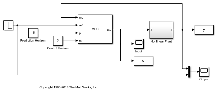
In the model, the MPC block has two inports where we can connect prediction horizon signal and control horizon signal. In each simulation, we vary the prediction horizon value (from 5 to 50) while keeping the control horizon at 4. We measure both the overshoot (%) and settling time (sec) from the saved simulation results. Note that the MPC controller object is not changed. Instead, the new horizon values are supplied as input signals at run-time.
p_choices = 5:5:50;
set_param([mdl '/Control Horizon'],'Value','4')
for p = p_choices
    set_param([mdl '/Prediction Horizon'],'Value',num2str(p))
    sim(mdl,20)
    settling_timeP(p/5) = ...
        find( ...
        (abs(y.signals.values-r0)<0.01) & ...
        (abs([0;diff(y.signals.values)]) < 0.001) ...
        ,1,'first')*Ts;
    if r0>y0
        overshootP(p/5) = abs((max(y.signals.values)-r0)/r0)*100;
    else
        overshootP(p/5) = abs((min(y.signals.values)-r0)/r0)*100;
    end
end
figure
subplot(2,1,1)
plot(p_choices,overshootP,'*')
xlabel('prediction horizon')
ylabel('overshoot (%)')
title('control horizon = 4')
subplot(2,1,2)
plot(p_choices,settling_timeP,'*')
ylabel('settling time (sec)')
xlabel('prediction horizon')
-->Converting model to discrete time.
-->Integrator added as output disturbance model for measured output #1.
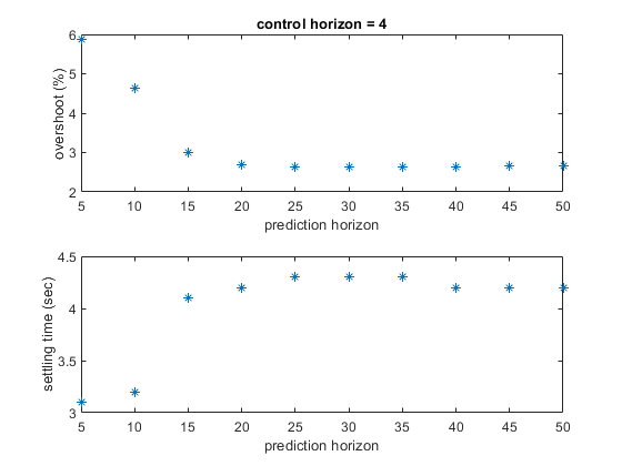
As the two plots show above, when prediction horizon increases from 5 to 15, the overshoot drops from 6% to 3% and settling time increases from 3 seconds to 4 seconds. After that, however, both overshoot and settling time remain more or less the same. In addition all the settling time values satisfy the upper bound of 5 seconds. Therefore, we choose the prediction horizon of 15, because it is the smallest value to achieve satisfactory performance by forming the smallest optimization problem.
Comparing Performance Between Different Control Horizon Choices
After we choose the prediction horizon, we use the same setup to evaluate different control horizon choices. In each simulation, we vary the control horizon (from 1 to 10) while keeping the prediction horizon at 15.
c_choices = 1:10;
set_param([mdl '/Prediction Horizon'],'Value','15')
for c = c_choices
    set_param([mdl '/Control Horizon'],'Value',num2str(c))
    sim(mdl,20)
    settling_timeC(c) = ...
        find( ...
        (abs(y.signals.values-r0)<0.01) & ...
        (abs([0;diff(y.signals.values)]) < 0.001) ...
        ,1,'first')*Ts;
    if r0>y0
        overshootC(c) = abs((max(y.signals.values)-r0)/r0)*100;
    else
        overshootC(c) = abs((min(y.signals.values)-r0)/r0)*100;
    end
end
figure
subplot(2,1,1)
plot(c_choices,overshootC,'*')
xlabel('control horizon')
ylabel('overshoot (%)')
title('prediction horizon = 15')
subplot(2,1,2)
plot(c_choices,settling_timeC,'*')
xlabel('control horizon')
ylabel('settling time (sec)')
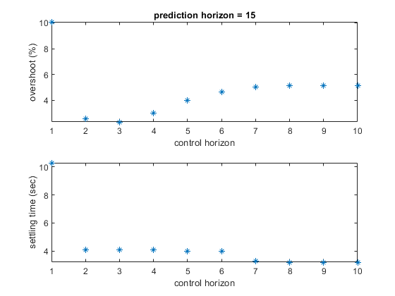
As the two plots show above, when control horizon increases from 1 to 3, the overshoot drops from 10% to 2%. After that, it increases back to 5% as control horizon grows from 4 to 10. The explanation is that when control horizon is 1, the controller doesn't have enough degrees of freedom to achieve reasonable response. When control horizon is 4 or beyond, the controller has more decision variables such that the first optimal move often becomes more aggressive and thus results in larger overshoot but shorter settling time. In this example, since the main control goal is to achieve minimum overshoot, we choose 3 as control horizon.
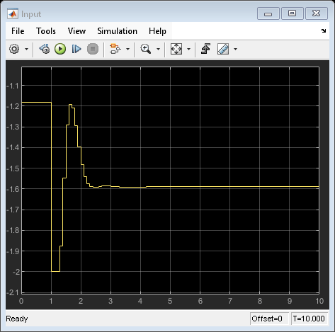
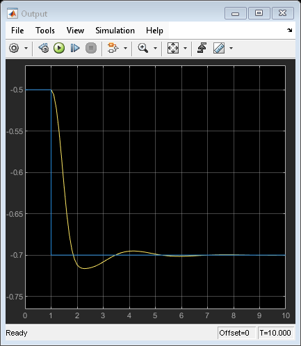
The model is simulated with prediction horizon = 15 and control horizon = 3. Recall that our original design choice is prediction horizon = 20 and control horizon = 4 based on a simple guideline, which is close to our final choice.
set_param([mdl '/Prediction Horizon'],'Value','15')
set_param([mdl '/Control Horizon'],'Value','3')
open_system([mdl '/Input'])
open_system([mdl '/Output'])
sim(mdl)
Adjusting Horizons in Real-Time on Embedded Systems
The major benefit of using run-time prediction and control horizon inports in MPC and Adaptive MPC blocks is that you can evaluate and adjust controller performance in real-time without regenerating code and re-deploying it to the target system. This feature is very helpful at the prototyping stage.
To use run-time horizon adjustment in real time, the target system must support dynamic memory allocation because as horizons change, the sizes of all that matrices used to construct the optimization problem change at run-time as well.
You also need to specify the maximum prediction horizon in the block dialog box to define the upper bound of the sizes of these matrices. Therefore, the memory footprint would be large. After finding the best horizon choices, it is recommended to disable the feature to have efficient code generation with fixed-size data.
See Also
Functions
linearize(Simulink Control Design)