Curve Fitting via Optimization
This example shows how to fit a nonlinear function to data. For this example, the nonlinear function is the standard exponential decay curve
where is the response at time , and and are the parameters to fit. Fitting the curve means finding parameters and that minimize the sum of squared errors
where the times are and the responses are . The sum of squared errors is the objective function.
Create Sample Data
Usually, you have data from measurements. For this example, create artificial data based on a model with and , with normally distributed pseudorandom errors.
rng default % for reproducibility
tdata = 0:0.1:10;
ydata = 40*exp(-0.5*tdata) + randn(size(tdata));
Write Objective Function
Write a function that accepts parameters A and lambda and data tdata and ydata, and returns the sum of squared errors for the model . Put all the variables to optimize (A and lambda) in a single vector variable (x). For more information, see Minimizing Functions of Several Variables.
type ssevalfunction sse = sseval(x,tdata,ydata) A = x(1); lambda = x(2); sse = sum((ydata - A*exp(-lambda*tdata)).^2);
Save this objective function as a file named sseval.m on your MATLAB® path.
The fminsearch solver applies to functions of one variable, x. However, the sseval function has three variables. The extra variables tdata and ydata are not variables to optimize, but are data for the optimization. Define the objective function for fminsearch as a function of x alone:
fun = @(x)sseval(x,tdata,ydata);
For information about including extra parameters such as tdata and ydata, see Parameterizing Functions.
Find the Best Fitting Parameters
Start from a random positive set of parameters x0, and have fminsearch find the parameters that minimize the objective function.
x0 = rand(2,1);
bestx = fminsearch(fun,x0)
bestx = 2×1

   40.6877
    0.4984
The result bestx is reasonably near the parameters that generated the data, A = 40 and lambda = 0.5.
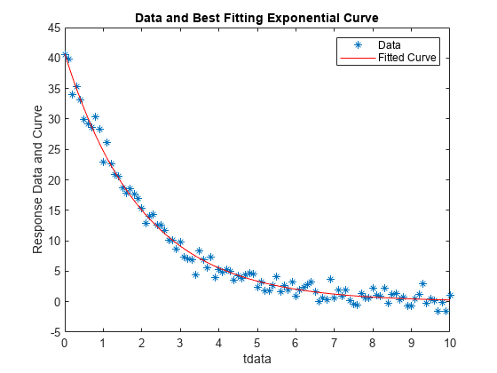
Check the Fit Quality
To check the quality of the fit, plot the data and the resulting fitted response curve. Create the response curve from the returned parameters of your model.
A = bestx(1);
lambda = bestx(2);
yfit = A*exp(-lambda*tdata);
plot(tdata,ydata,'*');
hold on
plot(tdata,yfit,'r');
xlabel('tdata')
ylabel('Response Data and Curve')
title('Data and Best Fitting Exponential Curve')
legend('Data','Fitted Curve')
hold off
See Also
Topics
- Optimizing Nonlinear Functions
- Nonlinear Data-Fitting (Optimization Toolbox)
- Nonlinear Regression (Statistics and Machine Learning Toolbox)