Data Smoothing and Outlier Detection
This example shows how to use data smoothing to eliminate unwanted noise or behaviors in data using the smoothdata function. This example also shows how to identify and handle outliers, which are data points that are significantly different from the rest of the data, using the isoutlier, filloutliers, or rmoutliers functions. Alternatively, you can interactively smooth noisy data and handle outliers in data using the Smooth Data and Clean Outlier Data tasks in the Live Editor.
Moving Window Methods
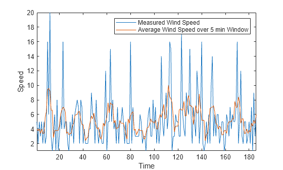
Moving window methods are ways to process data in smaller batches at a time, typically in order to statistically represent a neighborhood of points in the data. The moving average is a common data smoothing technique that slides a window along the data, computing the mean of the points inside of each window. This can help to eliminate insignificant variations from one data point to the next.
For example, consider wind speed measurements taken every minute for about 3 hours. Use the movmean function with a window size of 5 minutes to smooth out high-speed wind gusts.
load windData.mat
mins = 1:length(speed);
window = 5;
meanspeed = movmean(speed,window);
plot(mins,speed,mins,meanspeed)
axis tight
legend("Measured Wind Speed","Average Wind Speed over 5 min Window")
xlabel("Time")
ylabel("Speed")
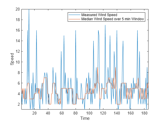
Similarly, you can compute the median wind speed over a sliding window using the movmedian function.
medianspeed = movmedian(speed,window);
plot(mins,speed,mins,medianspeed)
axis tight
legend("Measured Wind Speed","Median Wind Speed over 5 min Window")
xlabel("Time")
ylabel("Speed")
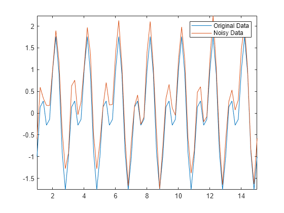
Not all data is suitable for smoothing with a moving window method. For example, create a sinusoidal signal with injected random noise.
t = 1:0.2:15;
A = sin(2*pi*t) + cos(2*pi*0.5*t);
Anoise = A + 0.5*rand(1,length(t));
plot(t,A,t,Anoise)
axis tight
legend("Original Data","Noisy Data")
Use a moving mean with a window size of 3 to smooth the noisy data.
window = 3;
Amean = movmean(Anoise,window);
plot(t,A,t,Amean)
axis tight
legend("Original Data","Moving Mean - Window Size 3")
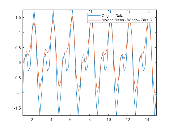
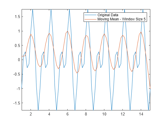
The moving mean achieves the general shape of the data, but doesn't capture the valleys (local minima) very accurately. Since the valley points are surrounded by two larger neighbors in each window, the mean is not a very good approximation to those points. If you make the window size larger, the mean eliminates the shorter peaks altogether. For this type of data, you might consider alternative smoothing techniques.
Amean = movmean(Anoise,5);
plot(t,A,t,Amean)
axis tight
legend("Original Data","Moving Mean - Window Size 5")
Common Smoothing Methods
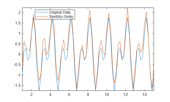
The smoothdata function provides several smoothing options such as the Savitzky-Golay method, which is a popular smoothing technique used in signal processing. By default, smoothdata chooses a best-guess window size for the method depending on the data.
Use the Savitzky-Golay method to smooth the noisy signal Anoise, and output the window size that it uses. This method provides a better valley approximation compared to movmean.
[Asgolay,window] = smoothdata(Anoise,"sgolay");
plot(t,A,t,Asgolay)
axis tight
legend("Original Data","Savitzky-Golay","location","best")
window
window =
3
The robust Lowess method is another smoothing method that is particularly helpful when outliers are present in the data in addition to noise. Inject an outlier into the noisy data, and use robust Lowess to smooth the data, which eliminates the outlier.
Anoise(36) = 20;
Arlowess = smoothdata(Anoise,"rlowess",5);
plot(t,Anoise,t,Arlowess)
axis tight
legend("Noisy Data","Robust Lowess")

Detecting Outliers
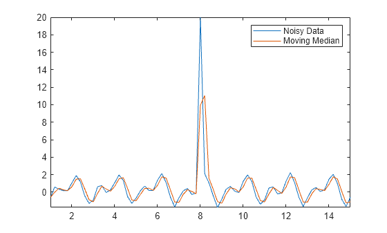
Outliers in data can significantly skew data processing results and other computed quantities. For example, if you try to smooth data containing outliers with a moving median, you can get misleading peaks or valleys.
Amedian = smoothdata(Anoise,"movmedian");
plot(t,Anoise,t,Amedian)
axis tight
legend("Noisy Data","Moving Median")
The isoutlier function returns a logical 1 when an outlier is detected. Verify the index and value of the outlier in Anoise.
TF = isoutlier(Anoise);
ind = find(TF)
ind =
36
Aoutlier = Anoise(ind)
Aoutlier =
20
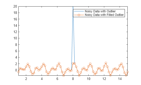
You can replace outliers in your data by using the filloutliers function and specifying a fill method. For example, fill the outlier in Anoise with the value of its neighbor immediately to the right.
Afill = filloutliers(Anoise,"next");
plot(t,Anoise,t,Afill,"o-")
axis tight
legend("Noisy Data with Outlier","Noisy Data with Filled Outlier")
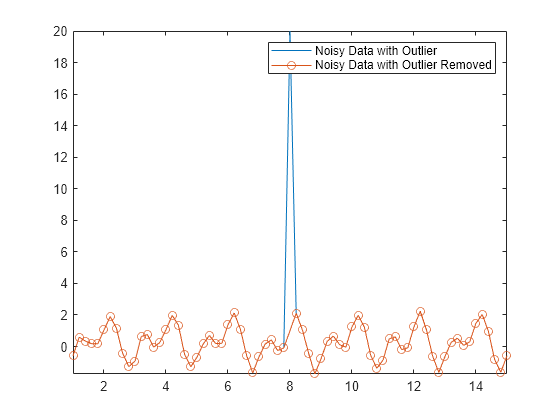
Alternatively, you can remove outliers from your data by using the rmoutliers function. For example, remove the outlier in Anoise.
Aremove = rmoutliers(Anoise);
plot(t,Anoise,t(~TF),Aremove,"o-")
axis tight
legend("Noisy Data with Outlier","Noisy Data with Outlier Removed")
Nonuniform Data
Not all data consists of equally spaced points, which can affect methods for data processing. Create a datetime vector that contains irregular sampling times for the data in Airreg. The time vector represents samples taken every minute for the first 30 minutes, then hourly over two days.
t0 = datetime(2014,1,1,1,1,1);
timeminutes = sort(t0 + minutes(1:30));
timehours = t0 + hours(1:48);
time = [timeminutes timehours];
Airreg = rand(1,length(time));
plot(time,Airreg)
axis tight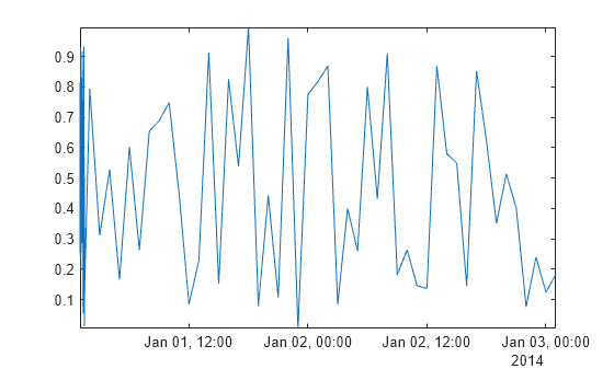
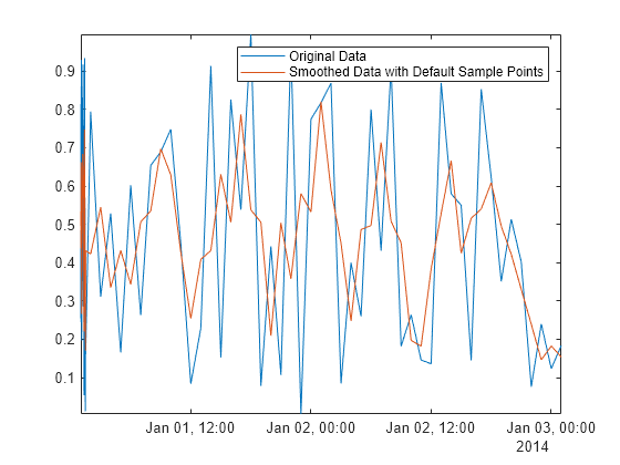
By default, smoothdata smooths with respect to equally spaced integers, in this case, 1,2,...,78. Since integer time stamps do not coordinate with the sampling of the points in Airreg, the first half hour of data still appears noisy after smoothing.
Adefault = smoothdata(Airreg,"movmean",3);
plot(time,Airreg,time,Adefault)
axis tight
legend("Original Data","Smoothed Data with Default Sample Points")
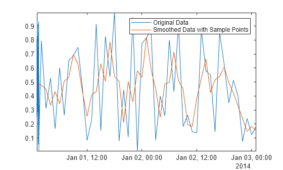
Many data processing functions in MATLAB®, including smoothdata, movmean, and filloutliers, allow you to provide sample points, ensuring that data is processed relative to its sampling units and frequencies. To remove the high-frequency variation in the first half hour of data in Airreg, use the SamplePoints name-value argument with the time stamps in time.
Asamplepoints = smoothdata(Airreg,"movmean", ...
    hours(3),"SamplePoints",time);
plot(time,Airreg,time,Asamplepoints)
axis tight
legend("Original Data","Smoothed Data with Sample Points")
See Also
Functions
smoothdata|isoutlier|filloutliers|rmoutliers|movmean|movmedian