Principal Component Analysis of Images

Since R2026a

Principal component analysis (PCA) is a statistical technique used to reduce the number of variables per sample, also known as the dimensionality, of large data sets while preserving as much important information as possible. In image processing, PCA transforms image data from the spatial domain into a new coordinate system defined by the principal components. The principal components represent the directions of maximum variance in the data. Thus, the principal components are the most informative directions in the data, enabling you to represent the data using only a few of them. This reduces the dimensionality of the data while retaining its key features.

You can use PCA to compress images without losing much visual quality, denoise images to remove low-variance components that often correspond to noise, or extract features within classification and segmentation applications. If you use PCA to extract features from a set of images, you can use those features to classify the category of each image. If you apply PCA to a single color image or a hyperspectral image, you can extract features of pixels for pixel classification and semantic segmentation. You can also use the extracted features as input to other machine learning and deep learning models. For an example of using PCA for image classification, see Identify Digits Using PCA for Feature Extraction.

This example shows how to apply principal component analysis to images. In this example, you perform these steps.

• Compute principal components from image data.

• Understand how the principal components represent information.

• Determine which components explain the most variability.

• Reconstruct the original data using the principal components.

Load Data Set

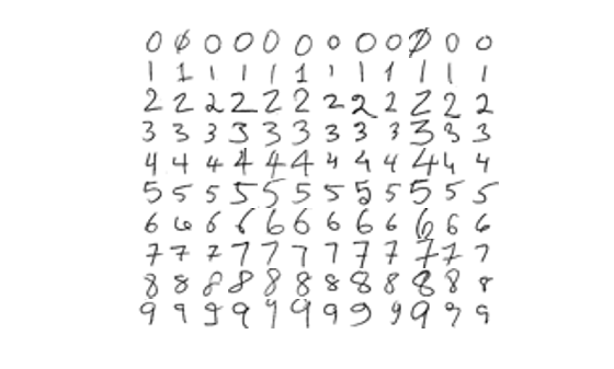
Load a data set of handwritten digits into the workspace as an image datastore.

handwrittenDir = fullfile(toolboxdir("vision"),"visiondata","digits","handwritten");
imds = imageDatastore(handwrittenDir,IncludeSubfolders=true,LabelSource="foldernames");

Visualize the data set.

figure
montage(imds,Size=[10 12])

Compute Principal Components

The PCA algorithm interprets each image as a high-dimensional vector data point. The datastore contains RGB images with three color channels, but the images do not have any color. Hence, convert the RGB images to grayscale images to remove the redundancy and reduce the dimension of the vector.

Reshape each image in the datastore as a vector of length p, where p is the number of pixels in the image. Create a matrix with n rows, where each row is a vectorized image from the datastore.

n = length(imds.Files);
I = readimage(imds,1);
I = im2gray(I);
[h,w] = size(I);
reset(imds)
p = h*w;
data = zeros(n,p);
for i = 1:n
    I = read(imds);
    I = im2gray(I);
    I = im2double(I);
    data(i,:) = reshape(I,1,[]);
end

The PCA algorithm subtracts the mean image from all images to center the data. Then, it captures the relationship between pixels by computing the covariance matrix of the centered data. The eigenvectors of this covariance matrix are the principal components. They represent the new axes that minimize the average projection cost between the data vectors and their projections.

The PCA algorithm projects the images onto these principal components to give a compact representation. You can interpret PCA as rotating your high-dimensional data vectors to align with the directions that best explain how your images differ from one another. The first principal component captures the most significant difference, the second captures the next most, and so on. In images, the first few components often capture large-scale patterns such as the general shape or orientation of the image, while later ones capture finer details or noise.

Apply PCA to the n-by-p matrix created from the vectorized images by using the pca (Statistics and Machine Learning Toolbox) function, and specify for the function to return these variables.

1. transformMatrix — A p-by-k matrix, where k is the number of principal components. Each row contains the principal component coefficients for a pixel of the image. The principal components form an orthogonal basis to the transform the image data.

2. transformedData – When you project a vectorized image onto the principal components, you get a transformed vectorized image that represents the weights of the principal components in the data. The transformedData matrix is an n-by-k matrix in which each row is a transformed vectorized image. Because the number of principal components k is typically much lower than the number of pixels p in the image, the transformed vectorized images typically have many fewer dimensions than pixels.

3. explainedVariability – A vector of length k in which each element represents the percentage of variability in the data set explained by the corresponding principal component.

4. mu – The mean vectorized image that the function subtracts from the data set to center the data.

[transformMatrix,transformedData,~,~,explainedVariability,mu] = pca(data);

Observe the percentage variability explained by the 119 principal components of the data set.

explainedVariability

explainedVariability = 119×1

    7.2708
    6.8159
    6.2647
    5.0638
    4.1678
    3.8515
    3.7323
    3.2083
    2.8895
    2.7465
    2.5750
    2.4795
    2.3417
    2.2315
    2.0425
      ⋮

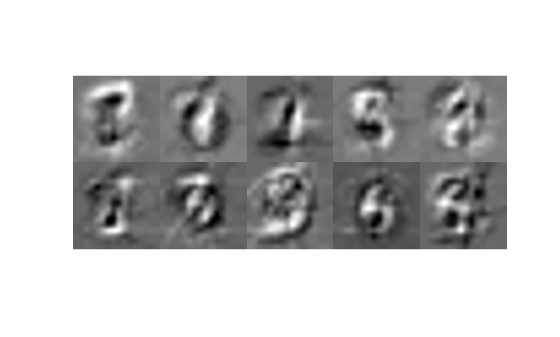
Visualize the first 10 principal components, which explain the highest percentage of variability in the data set. Observe that each principal component emphasizes a particular direction of variation of the handwritten digits.

pcImage = cell(1,10);
for i = 1:10
    principalComponent = transformMatrix(:,i);
    pcImage{i} = reshape(principalComponent,h,w);
    pcImage{i} = rescale(pcImage{i});
end
figure
montage(pcImage,Size=[2 5])

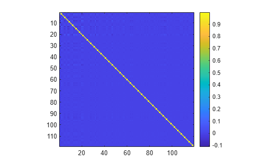
Visualize the cross-correlation between the principal components. Observe that all principal components are orthogonal to each other. Thus, each principal component represents an independent direction of variability and contributes uniquely to explaining the variance in the data.

pcacorr = corrcoef(transformMatrix);
figure
imagesc(pcacorr)
axis equal tight
colorbar

Reconstruct Images from Principal Components

You can completely describe the data set using the 119 principal components in transformMatrix, the transformed data transformedData, and the mean image mu as:

data = transformedData*transformMatrix' + mu

To preserve the essential characteristics of the data set in less space, retain only the principal components with the highest explained variability, and reconstruct the image using fewer principal components. For example, you can reconstruct the image using only the first k principal components as:

data = transformedData(:,1:k)*transformMatrix(:,1:k)' + mu

Adding the mean image mu back to the reconstruction prevents you from getting a dark reconstruction.

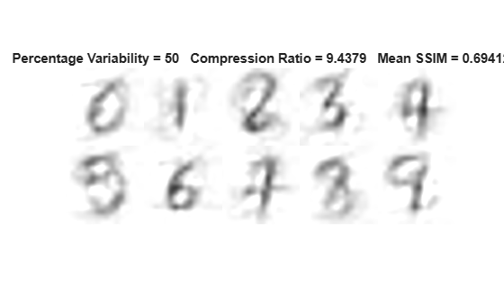
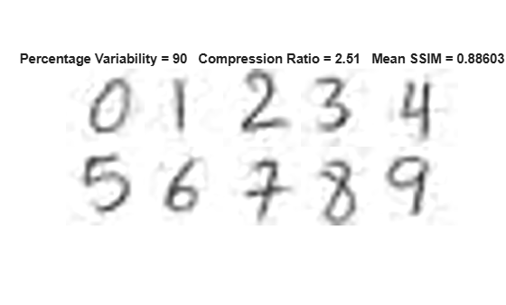
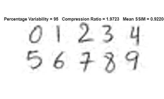
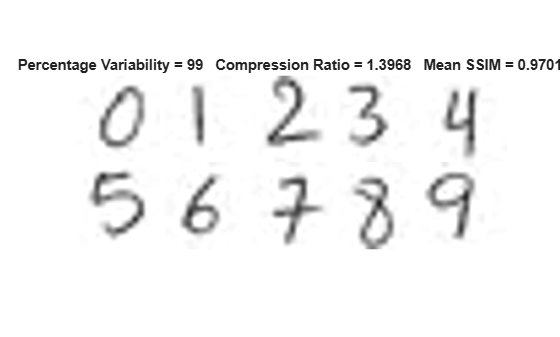
Find the number of principal components required to capture 50%, 90%, 95%, and 99% variability in the data set.

cumExplainedVariability = cumsum(explainedVariability);
reqdVariability = [50 90 95 99];
reducedDim = zeros(1,4);
for i = 1:4
    reducedDim(i) = find(cumExplainedVariability>reqdVariability(i),1);
    disp("Percentage Variability = " + reqdVariability(i));
    disp("Number of Dimensions = " + reducedDim(i));
end

Percentage Variability = 50

Number of Dimensions = 12

Percentage Variability = 90

Number of Dimensions = 47

Percentage Variability = 95

Number of Dimensions = 60

Percentage Variability = 99

Number of Dimensions = 85

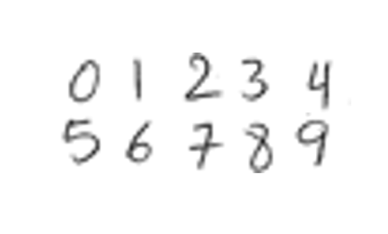
Visualize one image of each digit.

origImg = cell(1,10);
imgIdx = 1:12:120;
for i = 1:10
    idx = imgIdx(i);
    origImg{i} = reshape(data(idx,:),h,w);
end
figure
montage(origImg,Size=[2 5])

Then, visualize the same images reconstructed using principal components that explain 50%, 90%, 95%, and 99% variability in the data set, respectively. Observe that as the cumulative percentage variability explained by the principal components increases, the details in the reconstructed images increase, the structural similarity (SSIM) with respect to the original images increases, and the compression ratio decreases.

origStorageSize = numel(transformedData) + numel(transformMatrix) + numel(mu);

for i = 1:4
    numComponents = reducedDim(i);
    reducedTransformedData = transformedData(:,1:numComponents);
    reducedTransformMatrix = transformMatrix(:,1:numComponents);
    reconStorageSize = numel(reducedTransformedData) + numel(reducedTransformMatrix) + numel(mu);
    compressionRatio = origStorageSize/reconStorageSize;

    reconData = reducedTransformedData*reducedTransformMatrix' + mu;
    reconImg = cell(1,10);
    ssimVal = zeros(1,10);
    for j = 1:10
        idx = imgIdx(j);
        reconImg{j} = reshape(reconData(idx,:),h,w);
        ssimVal(j) = ssim(reconImg{j},origImg{j});
    end
    meanSSIM = mean(ssimVal);

    figure
    montage(reconImg,Size=[2 5])
    titleString = "Percentage Variability = " + reqdVariability(i) ...
                     + "   Compression Ratio = " + compressionRatio ...
                     + "   Mean SSIM = " + meanSSIM;
    title(titleString)
end

Further Exploration

If you have a data set of color images, separate the red, green, and blue channels, apply PCA to each channel separately, and then combine the results using a method suitable for your application.

• To compress or reduce the dimensionality of the data set, store the reduced number of principal components in the transform matrix and the reduced number of weights in the transformed data for each channel separately.

• To reconstruct the image from the reduced principal components, reconstruct each channel separately. Reconstruct the color image by concatenating the three reconstructed channels along the third dimension.

• To extract features for classification or segmentation applications, extract features for each channel separately. Use the collective set of features from all three channels to perform classification or segmentation.

For a single image with multiple channels, such as a hyperspectral images with hundreds of channels, you can apply PCA by using the hyperpca function. The hyperpca function considers the channels as the dimensions and each pixel as a data point. In this case, you can interpret the principal components as decorrelated channels because of their orthogonality. You can reduce the dimensionality of the hyperspectral image by using only the first few transformed channels for each pixel. You can also use the transformed channels as feature descriptors of each pixel for applications such as pixel classification and semantic segmentation.