What Are Hammerstein-Wiener Models?
When the output of a system depends nonlinearly on its inputs, sometimes it is possible to decompose the input-output relationship into two or more interconnected elements. In this case, you can represent the dynamics by a linear transfer function and capture the nonlinearities using nonlinear functions of inputs and outputs of the linear system. The Hammerstein-Wiener model achieves this configuration as a series connection of static nonlinear blocks with a dynamic linear block. Hammerstein-Wiener model applications span several areas, such as modeling electromechanical system and radio frequency components, audio and speech processing, and predictive control of chemical processes. These models have a convenient block representation, a transparent relationship to linear systems, and are easier to implement than heavy-duty nonlinear models such as neural networks and Volterra models.
You can use a Hammerstein-Wiener model as a black-box model structure because it provides a flexible parameterization for nonlinear models. For example, you can estimate a linear model and try to improve its fidelity by adding an input or output nonlinearity to this model. You can also use a Hammerstein-Wiener model as a grey-box structure to capture physical knowledge about process characteristics. For example, the input nonlinearity can represent typical physical transformations in actuators and the output nonlinearity can describe common sensor characteristics. For more information about when to fit nonlinear models, see About Identified Nonlinear Models.
Structure of Hammerstein-Wiener Models
Hammerstein-Wiener models describe dynamic systems using one or two static nonlinear blocks in series with a linear block. The linear block is a discrete transfer function that represents the dynamic component of the model.
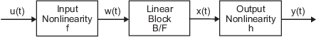
This block diagram represents the structure of a Hammerstein-Wiener model:
Where,
f is a nonlinear function that transforms input data u(t) as w(t) = f(u(t)).
w(t), an internal variable, is the output of the Input Nonlinearity block and has the same dimension as u(t).
B/F is a linear transfer function that transforms w(t) as x(t) = (B/F)w(t).
x(t), an internal variable, is the output of the Linear block and has the same dimension as y(t).
B and F are similar to polynomials in a linear Output-Error model. For more information about Output-Error models, see What Are Polynomial Models?
For ny outputs and nu inputs, the linear block is a transfer function matrix containing entries:
where j =
1,2,...,nyand i =1,2,...,nu.h is a nonlinear function that maps the output of the linear block x(t) to the system output y(t) as y(t) = h(x(t)).
Because f acts on the input port of the linear block, this function is called the input nonlinearity. Similarly, because h acts on the output port of the linear block, this function is called the output nonlinearity. If your system contains several inputs and outputs, you must define the functions f and h for each input and output signal. You do not have to include both the input and the output nonlinearity in the model structure. When a model contains only the input nonlinearity f, it is called a Hammerstein model. Similarly, when the model contains only the output nonlinearity h, it is called a Wiener model.
The software computes the Hammerstein-Wiener model output y in three stages:
Compute w(t) = f(u(t)) from the input data.
w(t) is an input to the linear transfer function B/F.
The input nonlinearity is a static (memoryless) function, where the value of the output a given time t depends only on the input value at time t.
You can configure the input nonlinearity as a sigmoid network, wavelet network, saturation, dead zone, piecewise linear function, one-dimensional polynomial, or a custom network. You can also remove the input nonlinearity.
Compute the output of the linear block using w(t) and initial conditions: x(t) = (B/F)w(t).
You can configure the linear block by specifying the orders of numerator B and denominator F.
Compute the model output by transforming the output of the linear block x(t) using the nonlinear function h as y(t) = h(x(t)).
Similar to the input nonlinearity, the output nonlinearity is a static function. You can configure the output nonlinearity in the same way as the input nonlinearity. You can also remove the output nonlinearity, such that y(t) = x(t).
Resulting models are idnlhw objects
that store all model data, including model parameters and nonlinearity
estimators. For more information about these objects, see Nonlinear Model Structures.
You can estimate Hammerstein-Wiener models in the System Identification app or at
the command line using the nlhw command.
You can use uniformly sampled time-domain input-output data for estimating
Hammerstein-Wiener models. Your data can have one or more input and
output channels. You cannot use time series data (output only) or
frequency-domain data for estimation. If you have time series data,
to fit a nonlinear model, identify nonlinear ARX models or nonlinear
grey-box models. For more information about these models, see Identifying Nonlinear ARX Models and Estimate Nonlinear Grey-Box Models.