Parameter and State Estimation in Simulink Using Particle Filter Block
This example demonstrates the use of the Particle Filter block in System Identification Toolbox™. A discrete-time transfer function parameter estimation problem is reformulated and recursively solved as a state estimation problem.
Introduction
The System Identification Toolbox has three Simulink® blocks for nonlinear state estimation:
Particle Filter: Implements a discrete-time particle filter algorithm.
Extended Kalman Filter: Implements the first-order discrete-time extended Kalman filter algorithm.
Unscented Kalman Filter: Implements the discrete-time unscented Kalman filter algorithm.
These blocks support state estimation using multiple sensors operating at different sample rates. A typical workflow for using these blocks is as follows:
Model your plant and sensor behavior using MATLAB® or Simulink functions.
Configure the parameters of the block.
Simulate the filter and analyze results to gain confidence in filter performance.
Deploy the filter on your hardware. You can generate code for these filters using Simulink Coder™ software.
This example uses the Particle Filter block to demonstrate the first two steps of this workflow. The last two steps are briefly discussed in the Next Steps section. The goal in this example is to estimate the parameters of a discrete-time transfer function (an output-error model) recursively, where the model parameters are updated at each time step as new information arrives.
If you are interested in the Extended Kalman Filter, see the example "Estimate States of Nonlinear System with Multiple, Multirate Sensors". The use of Unscented Kalman Filter follows similar steps to Extended Kalman Filter.
Plant Modeling
Most state estimation algorithms rely on a plant model (state transition function) that describes the evolution of plant states from one time step to the next. This function is typically denoted as ![$x[k+1]=f(x[k],w[k],u[k])$](../../examples/ident/win64/ParameterAndStateEstimationUsingParticleFilterBlockExample_eq06189551820484413923.png) where x is the states, w is the process noise, u is the optional additional inputs, for instance system inputs or parameters. The Particle Filter block requires you to provide this function in a slightly different syntax,
where x is the states, w is the process noise, u is the optional additional inputs, for instance system inputs or parameters. The Particle Filter block requires you to provide this function in a slightly different syntax, ![$X[k+1]=f_{pf}(X[k],u[k])$](../../examples/ident/win64/ParameterAndStateEstimationUsingParticleFilterBlockExample_eq16853415067683482667.png) . The differences are:
. The differences are:
Particle filter works by following the trajectories of many state hypotheses (particles), and the block passes all state hypotheses to your function at once. Concretely, if your state vector
 has
has  elements and you choose
  particles to use,
  has the dimensions
 ![$[N_s \; N_p]$](../../examples/ident/win64/ParameterAndStateEstimationUsingParticleFilterBlockExample_eq04825736176809034596.png) where each column is a state hypothesis.
where each column is a state hypothesis.You calculate the impact of process noise
 on the state hypotheses
 ![$X[k+1]$](../../examples/ident/win64/ParameterAndStateEstimationUsingParticleFilterBlockExample_eq02106988218071147168.png) in your function
in your function  . The block does not make any assumptions on the probability distribution of the process noise , and does not need as an input.
The function can be a MATLAB Function that complies with the restrictions of MATLAB Coder™, or a Simulink Function block. After you create , you specify the function name in the Particle Filter block.
In this example, you are reformulating a discrete-time transfer function parameter estimation problem as a state estimation problem. This transfer function may be representing the dynamics of a discrete-time process, or it may be representing some continuous-time dynamics coupled with a signal reconstructor such as zero-order hold. Assume that you are interested in estimating the parameters of a first-order discrete-time transfer function:
![$ y[k] = \frac{20q^{-1}}{1-0.7q^{-1}} u[k] + e[k] $](../../examples/ident/win64/ParameterAndStateEstimationUsingParticleFilterBlockExample_eq18371076909130355514.png) .
.
Here ![$y[k]$](../../examples/ident/win64/ParameterAndStateEstimationUsingParticleFilterBlockExample_eq11260577188396988852.png) is the plant output,
is the plant output, ![$u[k]$](../../examples/ident/win64/ParameterAndStateEstimationUsingParticleFilterBlockExample_eq03418053420324258546.png) is the plant input,
is the plant input, ![$e[k]$](../../examples/ident/win64/ParameterAndStateEstimationUsingParticleFilterBlockExample_eq04201606104284013941.png) is the measurement noise,
is the measurement noise,  is the time-delay operator so that
 ![$q^{-1}u[k]=u[t-1]$](../../examples/ident/win64/ParameterAndStateEstimationUsingParticleFilterBlockExample_eq17139541702203966118.png) . Parameterize the transfer function as
. Parameterize the transfer function as  , where
  and
and  are parameters to be estimated. The transfer function and the parameters can be represented in the necessary state-space form in multiple ways, by choice of the state vector. One choice is
 ![$x[k]=[\; y[k]; d[k]; n[k] \;]$](../../examples/ident/win64/ParameterAndStateEstimationUsingParticleFilterBlockExample_eq01979344277059616014.png) where the second and third states represent the parameter estimates. Then the transfer function can be equivalently written as
where the second and third states represent the parameter estimates. Then the transfer function can be equivalently written as
![$ x[k+1] = \left[ \begin{array}{c} -x_2[k] x_1[k] + x_3[k] u[k] \\ x_2[k] \\ x_3[k] \\ \end{array} \right] $](../../examples/ident/win64/ParameterAndStateEstimationUsingParticleFilterBlockExample_eq01945190232887644165.png) .
.
The measurement noise term is handled in sensor modeling. In this example, you implement the expression above in a MATLAB Function, in a vectorized form for computational efficiency:
type pfBlockStateTransitionFcnExample
function xNext = pfBlockStateTransitionFcnExample(x,u)
% pfBlockStateTransitionFcnExample State transition function for particle
%                                  filter, for estimating parameters of a
%                                  SISO, first order, discrete-time transfer
%                                  function model
%
% Inputs:
%    x - Particles, a NumberOfStates-by-NumberOfParticles matrix
%    u - System input, a scalar
%
% Outputs:
%    xNext - Predicted particles, with the same dimensions as input x

% Implement the state-transition function
%    xNext = [x(1)*x(2) + x(3)*u;
%             x(2);
%             x(3)];
% in vectorized form (for all particles).
xNext = x;
xNext(1,:) = bsxfun(@times,x(1,:),-x(2,:)) + x(3,:)*u;

% Add a small process noise (relative to expected size of each state), to
% increase particle diversity
xNext = xNext + bsxfun(@times,[1; 1e-2; 1e-1],randn(size(xNext)));
end
Sensor Modeling
The Particle Filter block requires you to provide a measurement likelihood function that calculates the likelihood (probability) of each state hypothesis. This function has the form ![$L[k] = h_{pf}(X[k],y[k],u[k])$](../../examples/ident/win64/ParameterAndStateEstimationUsingParticleFilterBlockExample_eq01334678795106168084.png) .
. ![$L[k]$](../../examples/ident/win64/ParameterAndStateEstimationUsingParticleFilterBlockExample_eq04435212642107953369.png) is an element vector, where is the number of particles you choose.
is an element vector, where is the number of particles you choose.  element in is the likelihood of the particle (column) in
 ![$X[k]$](../../examples/ident/win64/ParameterAndStateEstimationUsingParticleFilterBlockExample_eq07716299756804254322.png) . is the sensor measurement. is an optional input argument, which can differ from the inputs of the state transition function.
. is the sensor measurement. is an optional input argument, which can differ from the inputs of the state transition function.
The sensor measures the first state in this example. This example assumes that the errors between the actual and predicted measurements are distributed according to a Gaussian distribution, but any arbitrary probability distribution or some other method can be used to calculate the likelihoods. You create  , and specify the function name in the Particle Filter block.
type pfBlockMeasurementLikelihoodFcnExample;
function likelihood = pfBlockMeasurementLikelihoodFcnExample(particles, measurement)
% pfBlockMeasurementLikelihoodFcnExample Measurement likelihood function for particle filter
%
% The measurement is the first state
%
% Inputs:
%    particles   - A NumberOfStates-by-NumberOfParticles matrix
%    measurement - System output, a scalar
%
% Outputs:
%    likelihood - A vector with NumberOfParticles elements whose n-th
%                 element is the likelihood of the n-th particle

%#codegen

% Predicted measurement
yHat = particles(1,:);

% Calculate likelihood of each particle based on the error between actual
% and predicted measurement
%
% Assume error is distributed per multivariate normal distribution with
% mean value of zero, variance 1. Evaluate the corresponding probability
% density function
e = bsxfun(@minus, yHat, measurement(:)'); % Error
numberOfMeasurements = 1;
mu = 0; % Mean
Sigma = eye(numberOfMeasurements); % Variance
measurementErrorProd = dot((e-mu), Sigma \ (e-mu), 1);
c = 1/sqrt((2*pi)^numberOfMeasurements * det(Sigma));
likelihood = c * exp(-0.5 * measurementErrorProd);
end
Filter Construction
Configure the Particle Filter block for estimation. You specify the state transition and measurement likelihood function names, number of particles, and the initial distribution of these particles.
In the System Model tab of the block dialog box, specify the following parameters:
State Transition
Specify the state transition function,
pfBlockStateTransitionFcnExample, in Function. When you enter the function name and click Apply, the block detects that your function has an extra input, , and creates the input port StateTransitionFcnInputs. You connect your system input to this port.
Initialization
Specify
10000in Number of particles. Higher number of particles typically correspond to better estimation, at increased computational cost.Specify
Gaussianin Distribution to get an initial set of particles from a multivariate Gaussian distribution. Then specify[0; 0; 0]in Mean because you have three states and this is your best guess. Specifydiag([10 5 100])in Covariance to specify a large variance (uncertainty) in your guess for the third state, and smaller variance for the first two. It is critical that this initial set of particles are spread wide enough (large variance) to cover the potential true state.
Measurement 1
Specify the name of your measurement likelihood function,
pfBlockMeasurementLikelihoodFcnExample, in Function.
Sample Time
At the bottom of the block dialog box, enter 1 in Sample time. If you have a different sample time among state transition and measurement likelihood functions, or if you have multiple sensors with different sample times, these can be configured in the Block outputs, Multirate tab.
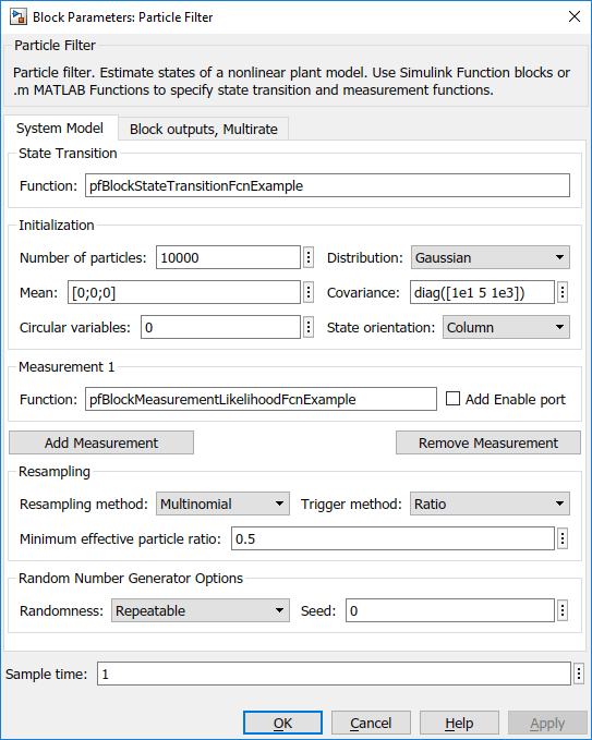
The particle filter involves deleting the particles with low likelihoods and seeding new particles using the ones with higher likelihoods. This is controlled by the options under the Resampling group. This example uses the default settings.
By default, the block only outputs the mean of the state hypotheses, weighted by their likelihoods. To see all the particles, weights, or to choose a different method of extracting a state estimate, check out the options in the Block outputs, Multirate tab.
Simulation and Results
For a simple test, the true plant model is simulated with white noise inputs. The inputs and the noisy measurements from the plant are fed to the Particle Filter block. The following Simulink model represents this setup.
open_system('pfBlockExample')
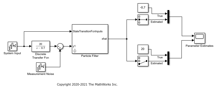
Simulate the system and compare the estimated and true parameters:
sim('pfBlockExample')
open_system('pfBlockExample/Parameter Estimates')

The plot shows the true numerator and denominator parameters, and their particle filter estimates. The estimates approximately converge to the true values after 10 time steps. Convergence is obtained even though the initial state guess was far from the true values.
Troubleshooting
A few potential implementation issues and troubleshooting ideas are listed here, in case the particle filter is not performing as expected for your application.
Troubleshooting of the particle filter is typically performed by looking into the set of particles and their weights, which can be obtained by choosing Output all particles and Output all weights in the Block outputs, Multirate tab of the block dialog box.
The first sanity check is to ensure that the state transition and measurement likelihood functions capture the behavior of your system reasonably well. If you have a simulation model for your system (and hence access to the true state in simulation), you can try initializing the filter with the true state. Then you can validate if the state transition function calculates the time-propagation of the true state accurately, and if the measurement likelihood function is calculating a high likelihood for these particles.
Initial set of particles is important. Ensure that at least some of the particles have high likelihood at the beginning of your simulation. If the true state is outside the initial spread of state hypotheses, the estimates can be inaccurate or even diverge.
If the state estimation accuracy is fine initially, but deteriorating over time, the issue may be particle degeneracy or particle impoverishment [2]. Particle degeneracy occurs when the particles are distributed too widely, while particle impoverishment occurs because of particles clumping together after resampling. Particle degeneracy leads to particle impoverishment as a result of direct resampling. The addition of artificial process noise in the state-transition function used in this example is one practical approach. There is a large collection of literature on resolving these issues and based on your application more systematic approaches may be available. [1], [2] are two references that can be helpful.
Next Steps
Validate the state estimation: Once the filter is performing as expected in a simulation, typically the performance is further validated using extensive Monte Carlo simulations. For more information, see Validate Online State Estimation in Simulink. You can use the options under Randomness group in the Particle Filter block dialog box to facilitate these simulations.
Generate code: The Particle Filter block supports C and C++ code generation using Simulink Coder software. The functions you provide to this block must comply with the restrictions of MATLAB Coder software (if you are using MATLAB functions to model your system) and Simulink Coder software (if you are using Simulink Function blocks to model your system).
Summary
This example has shown how to use the Particle Filter block in System Identification Toolbox. You estimated the parameters of a discrete-time transfer function recursively, where the parameters are updated at each time step as new information arrives.
close_system('pfBlockExample',0)
References
[1] Simon, Dan. Optimal state estimation: Kalman, H infinity, and nonlinear approaches. John Wiley & Sons, 2006.
[2] Doucet, Arnaud, and Adam M. Johansen. "A tutorial on particle filtering and smoothing: Fifteen years later." Handbook of nonlinear filtering 12.656-704 (2009): 3.
See Also
Extended Kalman Filter | Unscented Kalman Filter | Particle Filter