Online ARMAX Polynomial Model Estimation
This example shows how to implement an online polynomial model estimator. You estimate two ARMAX models for a nonlinear chemical reaction process. These models capture the behavior of the process at two operating conditions. The model behavior is identified online and used to adjust the gains of an adaptive PI controller during system operation.
Continuously Stirred Tank Reactor
A Continuously Stirred Tank Reactor (CSTR) is a common chemical system in the process industry. A schematic of the CSTR system is:

This is a jacketed diabatic (i.e., nondiabatic) tank reactor described extensively in Bequette's book "Process Dynamics: Modeling, Analysis and Simulation", published by Prentice-Hall, 1998. The vessel is assumed to be perfectly mixed, and a single first-order exothermic and irreversible reaction, A --> B, takes place. The inlet stream of reagent A is fed to the tank at a constant rate. After stirring, the end product streams out of the vessel at the same rate as reagent A is fed into the tank (the volume in the reactor tank is constant). Details of the operation of the CSTR and its 2-state nonlinear model used in this example are explained in the example Non-Adiabatic Continuous Stirred Tank Reactor: MATLAB File Modeling with Simulations in Simulink.
The inputs of the CSTR model are:
![$$ \begin{array} {ll} u_1(t) = C_{Af}(t) \; & \textnormal{Concentration of A in inlet feed stream} [kgmol/m^3] \\ u_2(t) = T_f(t) \; & \textnormal{Inlet feed stream temperature} [K] \\ u_3(t) = T_j(t) \; & \textnormal{Jacket coolant temperature} [K] \\ \end{array} $$](../../examples/ident/win64/OnlinePolynomialModelEstimationExample_eq14776539609272759793.png)
and the outputs (y(t)), which are also the states of the model (x(t)), are:
![$$ \begin{array} {ll} y_1(t) = x_1(t) = C_{A}(t) \; & \textnormal{Concentration of A in reactor tank} [kgmol/m^3] \\ y_2(t) = x_2(t) = T(t) \; & \textnormal{Reactor temperature} [K] \\ \end{array} $$](../../examples/ident/win64/OnlinePolynomialModelEstimationExample_eq13140510021428426088.png)
The control objective is to maintain the concentration of reagent A,  at the desired level
  , which changes over time. The jacket temperature
  is manipulated by a PI controller in order to reject disturbances arising from the inlet feed stream temperature
  . The input of the PI controller is the tracking error signal,
  . The inlet feed stream concentration,
  , is assumed to be constant. The Simulink® model
 iddemo_cstr implements the CSTR plant as the block CSTR.
open_system('iddemo_cstr');

The  feed temperature input consists of a white noise disturbance on top of a constant offset. The noise power is 0.0075 [K^2]. This noise level causes up to 2% deviation from the desired
  .
.
The  signal in this example contains a step change from 1.5 [kgmol/m^3] to 2 [kgmol/m^3] at time
  . In addition to this step change,
  also contains a white noise perturbation for t in the [0,200) and [400,600) ranges. The power of this white noise signal is 0.015. The noise power is adjusted empirically to approximately give a signal-to-noise ratio of 10. Not having sufficient excitation in the reference signal in closed-loop identification can lead to not having sufficient information to identify a unique model. The implementation of
  is in the
 iddemo_cstr/CA Reference block.
Online Estimation for Adaptive Control
It is known from the nonlinear model that the CSTR output  is more sensitive to the control input
  at higher
  levels. The Recursive Polynomial Model Estimator block is used to detect this change in sensitivity. This information is used to adjust the gains of the PI controller as
  varies. The aim is to avoid having a high gain control loop which may lead to instability.
You estimate a discrete transfer-function from  to
to  online with the Recursive Polynomial Model Estimator block. The adaptive control algorithm uses the DC gain of this transfer function. The tracking error
  , is divided by the normalized DC gain of the estimated transfer function. This normalization is done to have a gain of 1 on the tracking error at the initial operating point, for which the PI controller is designed. For instance, the error signal is divided by 2 if the DC gain becomes 2 times its original value. This corresponds to dividing the PI controller gains by 2. This adaptive controller is implemented in
 iddemo_cstr/Adaptive PI Controller.
Recursive Polynomial Model Estimator Block Inputs
The 'Recursive Polynomial Model Estimator' block is found under the System Identification Toolbox/Estimators library in Simulink. You use this block to estimate linear models with ARMAX structure. ARMAX models have the form:
![$$ \begin{array} {l}A(q)\bar{y}(t)=B(q)\bar{u}(t)+C(q)\bar{e}(t) \\[0.1in] A(q) = 1+a_1z^{-1}+a_2z^{-2}+\cdots+a_{na}z^{-na} \\ B(q) = (b_01+b_1z^{-1}+b_2z^{-2}+\cdots+a_{nb-1}z^{-nb+1})z^{-nk} \\ C(q) = 1+c_1z^{-1}+c_2z^{-2}+\cdots+c_{nc}z^{-nc} \\ \end{array} $$](../../examples/ident/win64/OnlinePolynomialModelEstimationExample_eq03440919189447996122.png)
The
InputsandOutputinport of the recursive polynomial model estimator block correspond to and
and  respectively. For the CSTR model
  and
and  are deviations from the jacket temperature and A concentration trim operating points:
  ,
,  . It is good to scale
  and
and  to have a peak amplitude of 1 to improve the numerical condition of the estimation problem. The trim operating points,
  and
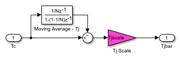
and  , are not known exactly before system operation. They are estimated and extracted from the measured signals by using a first-order moving average filter. These preprocessing filters are implemented in the
 iddemo_cstr/Preprocess Tjandiddemo_cstr/Preprocess CAblocks.
open_system('iddemo_cstr/Preprocess Tj');
The optional
Enableinport of the Recursive Polynomial Model Estimator block controls the parameter estimation in the block. Parameter estimation is disabled when the Enable signal is zero. Parameter estimation is enabled for all other values of theEnablesignal. In this example the estimation is disabled for the time intervals and
and  . During these intervals the measured input
  does not contain sufficient excitation for closed-loop system identification.
Recursive Polynomial Model Estimator Block Setup
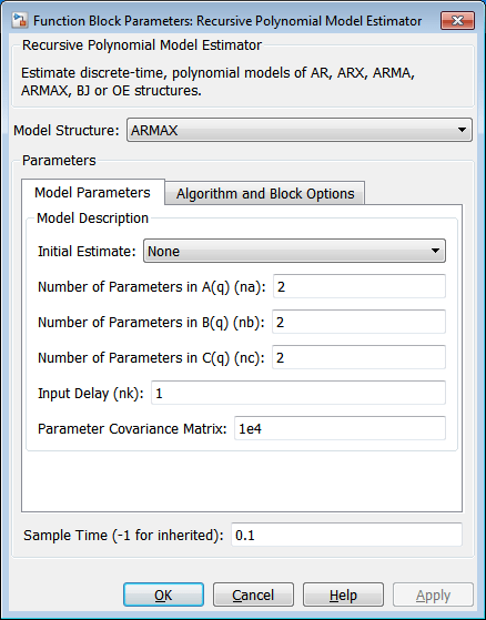
Configure the block parameters to estimate a second-order ARMAX model. In the Model Parameters tab, specify:
Model Structure: ARMAX. Choose ARMAX since the current and past values of the disturbances acting on the system,
 , are expected to impact the CSTR system output
  .
.
Initial Estimate: None. By default, the software uses a value of 0 for all estimated parameters.
Number of parameters in A(q) (na):
2. The nonlinear model has 2 states.
Number of parameters in B(q) (nb):
2.
Number of parameters in C(q) (nc):
2. The estimated model corresponds to a second order model since the maximum of na, nb, and nc are 2.
Input Delay (nk):
1. Like most physical systems, the CSTR system does not have direct feedthrough. Also, there are no extra time delays between its I/Os.
Parameter Covariance Matrix:
1e4. Specify a high covariance value because the initial guess values are highly uncertain.
Sample Time:
0.1. The CSTR model is known to have a bandwidth of about 0.25Hz. chosen such that 1/0.1 is greater than 20 times this bandwidth (5Hz).
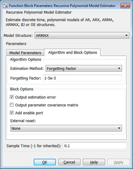
Click Algorithm and Block Options to set the estimation options:
Estimation Method:
Forgetting Factor
Forgetting Factor:
1-5e-3. Since the estimated parameters are expected to change with the operating point, set the forgetting factor to a value less than 1. Choose which corresponds to a memory time constant of
  seconds. A 100 second memory time ensures that a significant amount data used for identification is coming from the 200 second identification period at each operating point.
Select the Output estimation error check box. You use this block output to validate the estimation.
Select the Add enable port check box. You only want to adapt the estimated model parameters when extra noise is injected in the reference port. The parameter estimation n is disabled through this port when the extra noise is no longer injected.
External reset:
None.
Recursive Polynomial Model Estimator Block Outputs
At every time step, the recursive polynomial model estimator provides an estimate for  ,
,  ,
,  , and the estimation error
  . The
. The Error outport of the polynomial model estimator block contains  and is also known as the one-step-ahead prediction error. The
 Parameters outport of the block contains the A(q), B(q), and C(q) polynomial coefficients in a bus signal. Given the chosen polynomial orders ( ,
,  ,
,  ,
,  ) the
) the Parameters bus elements contain:
![$$ \begin{array} {l} A(t) = [1 \; a_1(t) \; a_2(t)] \\ B(t) = [0 \; b_0(t) \; b_1(t)] \\ C(t) = [1 \; c_1(t) \; c_2(t)] \\ \end{array} $$](../../examples/ident/win64/OnlinePolynomialModelEstimationExample_eq01674863182201742135.png)
The estimated parameters in the A(q), B(q), and C(q) polynomials change during simulation as follows:
sim('iddemo_cstr');
close_system('iddemo_cstr/Preprocess Tj');
open_system('iddemo_cstr/ABC');
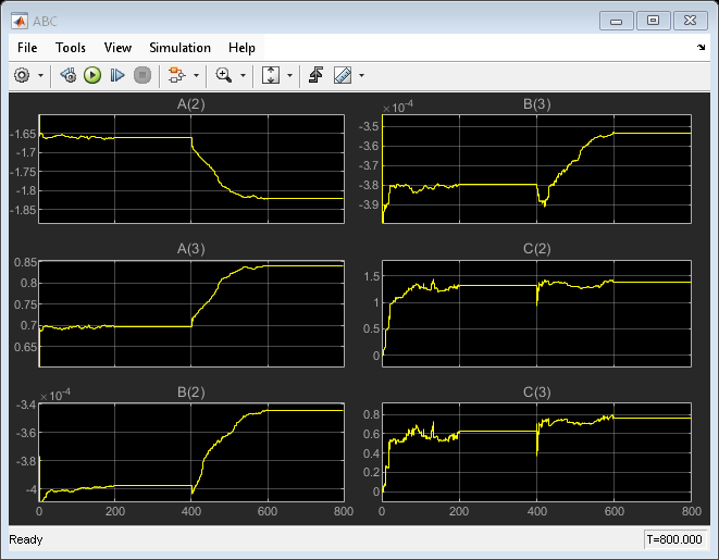
The parameter estimates quickly change from their initial values of 0 due to the high value chosen for the initial parameter covariance matrix. The parameters in the  and
and  polynomials approach their values at
  rapidly. However, the parameters in the
  polynomial show some fluctuations. One reason behind these fluctuations is that the disturbance
  to CSTR output
  is not fully modeled by the ARMAX structure. The error model
  is not important for the control problem studied here since the
  to
to  relationship is captured by the transfer function
  . Therefore, the fluctuation in
  is not a concern for this identification and control problem.
The parameter estimates are held constant for  since the estimator block was disabled for this interval (0 signal to the
 Enable inport). The parameter estimation is enabled at  when the CSTR tank starts switching to its new operating point. The parameters of
  and
and  converge to their new values by
  , and then held constant by setting the
 Enable port to 0. The convergence of  and
and  is slower at this operating point. This slow convergence is because of the smaller eigenvalues of the parameter covariance matrix at t=400 compared to the initial 1e4 values set at t=0. The parameter covariance, which is a measure of confidence in the estimates, is updated with each time step. The algorithm quickly changed the parameter estimates when the confidence in estimates were low at t=0. The improved parameter estimates capture the system behavior better, resulting in smaller one-step-ahead prediction errors and smaller eigenvalues in the parameter covariance matrix (increased confidence). The system behavior changes in t=400. However, the block is slower to change the parameter estimates due to the increased confidence in the estimates. You can use the External Reset option of the Recursive Polynomial Model Estimator block to provide a new value for parameter covariance at t=400. To see the value of the parameter covariance, select the Output parameter covariance matrix check box in the Recursive Polynomial Model Estimator block.
Validating the Estimated Model
The Error output of the Recursive Polynomial Model Estimator block gives the one-step-ahead error for the estimated model.
close_system('iddemo_cstr/ABC');
open_system('iddemo_cstr/1-Step Ahead Prediction Error');
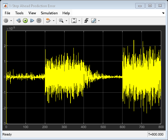
The one-step-ahead error is higher when there are no extra perturbations injected in the  channel for system identification. These higher errors may be caused by the lack of sufficient information in the
  input channel that the estimator block relies on. However, even this higher error is low and bounded when compared to the measured fluctuations in
  . This gives confidence in the estimated parameter values.
A more rigorous check of the estimated model is to simulate the estimated model and compare with the actual model output. The iddemo_cstr/Time-Varying ARMAX block implements the time-varying ARMAX model estimated by the Online Polynomial Model Estimator block. The error between the output of the CSTR system and the estimated time-varying ARMAX model output is:
close_system('iddemo_cstr/1-Step Ahead Prediction Error');
open_system('iddemo_cstr/Simulation Error');
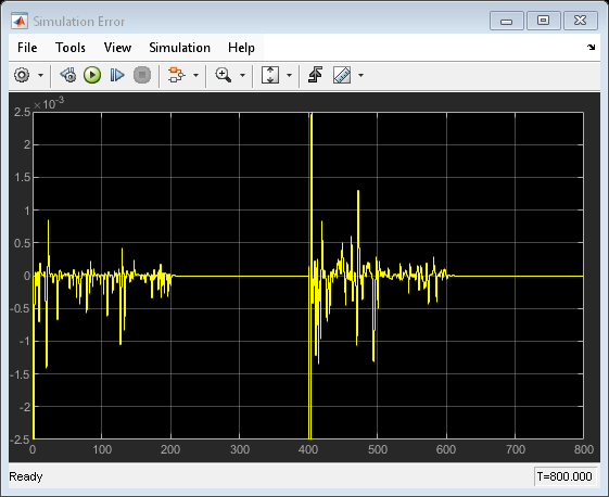
The simulation error is again bounded and low when compared to the fluctuations in the  . This further provides confidence that the estimated linear models are able to predict the nonlinear CSTR model behavior.
The identified models can be further analyzed in MATLAB. The model estimates for the operating points ![$C_A=1.5 [kgmol/m^3]$](../../examples/ident/win64/OnlinePolynomialModelEstimationExample_eq01145996814064713081.png) and
and ![$C_A=2 [kgmol/m^3]$](../../examples/ident/win64/OnlinePolynomialModelEstimationExample_eq14862851650486291760.png) can be obtained by looking at the estimated A(q), B(q), and C(q) polynomials at
can be obtained by looking at the estimated A(q), B(q), and C(q) polynomials at  and
and  respectively. Bode plots of these models are:
Ts = 0.1;
tidx = find(t>=200,1);
P200 = idpoly(AHat(:,:,tidx),BHat(:,:,tidx),CHat(:,:,tidx),1,1,[],Ts);
tidx = find(t>=600,1);
P600 = idpoly(AHat(:,:,tidx),BHat(:,:,tidx),CHat(:,:,tidx),1,1,[],Ts);
bodemag(P200,'b',P600,'r--',{10^-1,20});
legend('Estimated Model at C_A=1.5 [kgmol/m^3]', ...
       'Estimated Model at C_A=2.0 [kgmol/m^3]', ...
       'Location', 'Best');
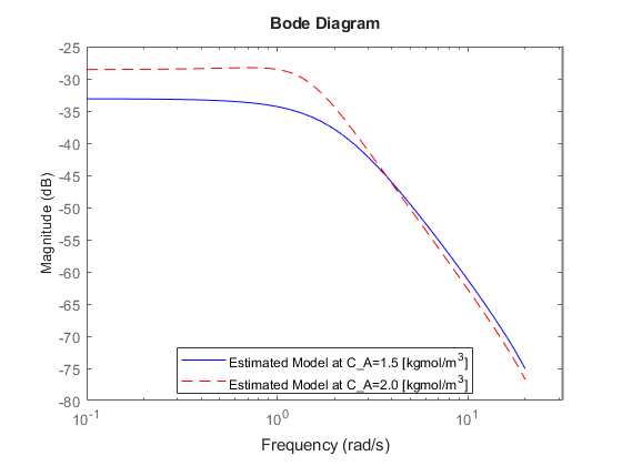
The estimated model has a higher gain at higher concentration levels. This is in agreement with prior knowledge about the nonlinear CSTR plant. The transfer function at ![$C_A(t)=2 [kgmol/m^3]$](../../examples/ident/win64/OnlinePolynomialModelEstimationExample_eq12994556848104239236.png) has a
has a  higher gain (double the amplitude) at low frequencies.
Summary
You estimated two ARMAX models to capture the behavior of the nonlinear CSTR plant at two operating conditions. The estimation was done during closed-loop operation with an adaptive controller. You looked at two signals to validate the estimation results: One step ahead prediction errors and the errors between the CSTR plant output and the simulation of the estimation model. Both of these errors signals were bounded and small compared to the CSTR plant output. This provided confidence in the estimated ARMAX model parameters.
bdclose('iddemo_cstr');