Glass Tube Manufacturing Process
This example shows linear model identification of a glass tube manufacturing process. The experiments and the data are discussed in:
V. Wertz, G. Bastin and M. Heet: Identification of a glass tube drawing bench. Proc. of the 10th IFAC Congress, Vol 10, pp 334-339 Paper number 14.5-5-2. Munich August 1987.
The output of the process is the thickness and the diameter of the manufactured tube. The inputs are the air-pressure inside the tube and the drawing speed.
The problem of modeling the process from the input speed to the output thickness is described below. Various options for analyzing data and determining model order are discussed.
Experimental Data
We begin by loading the input and output data, saved as an iddata object:
load thispe25.matThe data are contained in the variable glass:
glass
glass =
Time domain data set with 2700 samples.
Sample time: 1 seconds

Outputs      Unit (if specified)
   Thickn

Inputs       Unit (if specified)
   Speed

Data Properties
Data has 2700 samples of one input (Speed) and one output (Thickn). The sample time is 1 sec.
For estimation and cross-validation purpose, split it into two halves:
ze = glass(1001:1500); %Estimation data
zv = glass(1501:2000,:); %Validation data
A close-up view of the estimation data:
plot(ze(101:200)) %Plot the estimation data range from samples 101 to 200.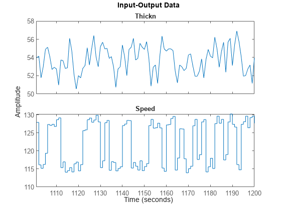
Preliminary Analysis of Data
Let us remove the mean values as a first preprocessing step:
ze = detrend(ze);
zv = detrend(zv);
The sample time of the data is 1 second, while the process time constants might be much slower. We may detect some rather high frequencies in the output. In order to affirm this, let us first compute the input and output spectra:
sy = spa(ze(:,1,[]));
su = spa(ze(:,[],1));
clf
spectrum(sy,su)
axis([0.024 10 -5 20])
legend({'Output','Input'})
grid on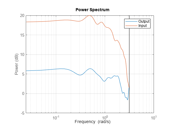
Note that the input has very little relative energy above 1 rad/sec while the output contains relatively larger values above that frequency. There are thus some high frequency disturbances that may cause some problem for the model building.
We compute the impulse response, using part of the data to gain some insight into potential feedback and delay from input to output (for delay estimation, it is recommended to set the RegularizationKernel to "none").
Imp = impulseest(ze,[],'negative',impulseestOptions(RegularizationKernel='none'));
showConfidence(impulseplot(Imp,-10:30),3)
grid on
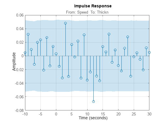
We see a delay of about 12 samples in the impulse response (first significant response value outside the confidence interval), which is quite substantial. Also, the impulse response is not insignificant for negative time lags. This indicates that there is a good probability of feedback in the data, so that future values of output influence (get added to) the current inputs. The input delay may be calculated explicitly using delayest:
delayest(ze)
ans =
12
The probability of feedback may be obtained using checkFeedback:
checkFeedback(ze) %compute probability of feedback in dataans = 100
Thus, it is almost certain that there is feedback present in the data.
We also, as a preliminary test, compute the spectral analysis estimate:
g = spa(ze);
showConfidence(bodeplot(g))
grid on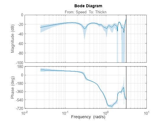
We note, among other things, that the high frequency behavior is quite uncertain. It may be advisable to limit the model range to frequencies lower than 1 rad/s.
Parametric Models of the Process Behavior
Let us do a quick check if we can pick up good dynamics by just computing a fourth order ARX model using the estimation data and simulate that model using the validation data. We know that the delay is about 12 seconds.
m1 = arx(ze,[4 4 12]);
compare(zv,m1);

A close view of simulation results:
compare(zv,m1,inf,'Samples',101:200)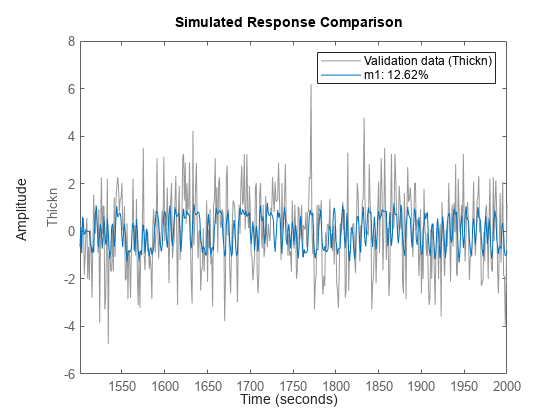
There are clear difficulties to deal with the high frequency components of the output. That, in conjunction with the long delay, suggests that we decimate the data by four (i.e. low-pass filter it and pick every fourth value):
zd = idresamp(detrend(glass),[1,4],20);

zde = zd(1:500);
zdv = zd(501:size(zd,'N'));
Let us find a good structure for the decimated data. First compute the impulse response:
Imp = impulseest(zde);
showConfidence(impulseplot(Imp,200),3)
axis([0  100  -0.05  0.01])
grid on
We again see that the delay is about 3 samples (which is consistent with what we saw above; 12 second delay with sample time of 4 seconds in zde). Let us now try estimating a default model, where the order is automatically picked by the estimator.
Mdefault = n4sid(zde);
compare(zdv,Mdefault)
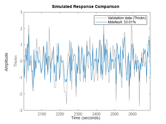
The estimator picked a 4th order model. It seems to provide a better fit than that for the undecimated data. Let us now systematically evaluate what model structure and orders we can use. First we look for the delay:
V = arxstruc(zde,zdv,struc(2,2,1:30));
nn = selstruc(V,0)
nn = 1×3

     2     2     3
ARXSTRUC also suggests a delay of 3 samples which is consistent with the observations from the impulse response. Therefore, we fix the delay to the vicinity of 3 and test several different orders with and around this delay:
V = arxstruc(zde,zdv,struc(1:5,1:5,nn(3)-1:nn(3)+1));
Now we call selstruc on the returned matrix in order to pick the most preferred model order (minimum loss function, which is shown in the first row of V).
nn = selstruc(V,0); %choose the "best" model orderSELSTRUC could be called with just one input to invoke an interactive mode of order selection (nn = selstruc(V)).
Let us compute and check the model for the "best" order returned in variable nn:
m2 = arx(zde,nn);
compare(zdv,m2,inf,compareOptions('Samples',21:150));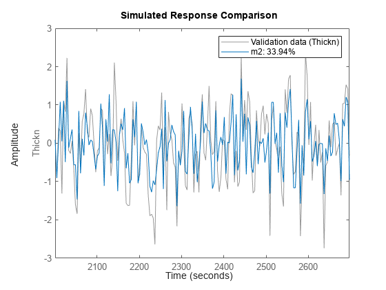
The model m2 is about same as Mdefault is fitting the data but uses lower orders.
Let us test the residuals:
resid(zdv,m2);
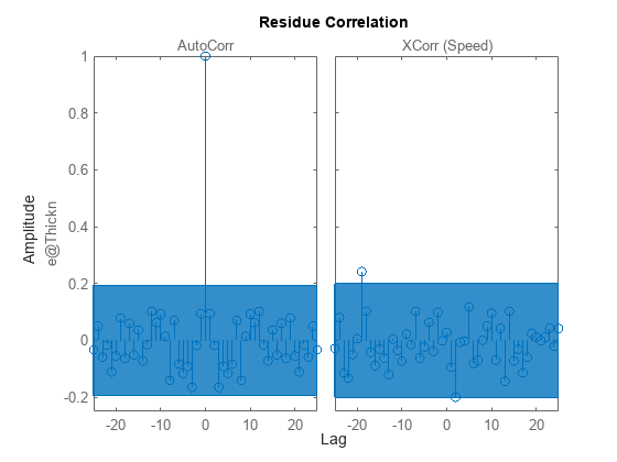
The residuals are inside the confidence interval region, indicating that the essential dynamics have been captured by the model. What does the pole-zero diagram tell us?
clf
showConfidence(iopzplot(m2),3)
axis([ -1.1898,1.3778,-1.5112,1.5688])
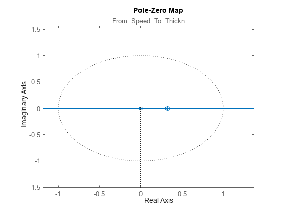
From the pole-zero plot, there is am indication of pole-zero cancellations for several pairs. This is because their locations overlap, within the confidence regions. This shows that we should be able to do well with lower order models. Try a [1 1 3] ARX model:
m3 = arx(zde,[1 1 3])
m3 =
Discrete-time ARX model: A(z)y(t) = B(z)u(t) + e(t)
  A(z) = 1 - 0.1236 z^-1

  B(z) = -0.1778 z^-3

Sample time: 4 seconds

Parameterization:
   Polynomial orders:   na=1   nb=1   nk=3
   Number of free coefficients: 2
   Use "polydata", "getpvec", "getcov" for parameters and their uncertainties.

Status:
Estimated using ARX on time domain data "zde".
Fit to estimation data: 35% (prediction focus)
FPE: 0.4362, MSE: 0.431

Model Properties
Simulation of model m3 compared against the validation data shows:
compare(zdv,Mdefault,m2,m3)
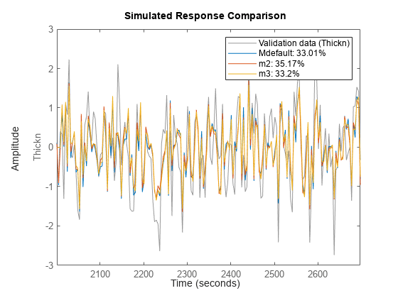
The three models deliver comparable results. Similarly, we can compare the 5-step ahead prediction capability of the models:
compare(zdv,Mdefault,m2,m3,5)
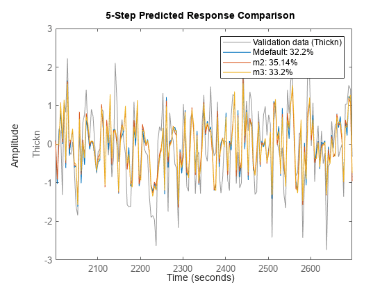
As these plots indicate, a reduction in model order does not significantly reduce its effectiveness is predicting future values.