Comparison of Various Model Identification Methods
This example shows several identification methods available in System Identification Toolbox™. We begin by simulating experimental data and use several estimation techniques to estimate models from the data. The following estimation routines are illustrated in this example: spa, ssest, tfest, arx, oe, armax and bj.
System Description
A noise corrupted linear system can be described by:
y = G u + H e
where y is the output and u is the input, while e denotes the unmeasured (white) noise source. G is the system's transfer function and H gives the description of the noise disturbance.
There are many ways to estimate G and H. Essentially they correspond to different ways of parameterizing these functions.
Defining a Model
System Identification Toolbox provides users with the option of simulating data as would have been obtained from a physical process. Let us simulate the data from an IDPOLY model with a given set of coefficients.
B = [0 1 0.5];
A = [1 -1.5 0.7];
m0 = idpoly(A,B,[1 -1 0.2],'Ts',0.25,'Variable','q^-1'); % The sample time is 0.25 s.
The third argument [1 -1 0.2] gives a characterization of the disturbances that act on the system. Execution of these commands produces the following discrete-time idpoly model:
m0
m0 =
Discrete-time ARMAX model: A(q)y(t) = B(q)u(t) + C(q)e(t)
  A(q) = 1 - 1.5 q^-1 + 0.7 q^-2

  B(q) = q^-1 + 0.5 q^-2

  C(q) = 1 - q^-1 + 0.2 q^-2

Sample time: 0.25 seconds

Parameterization:
   Polynomial orders:   na=2   nb=2   nc=2   nk=1
   Number of free coefficients: 6
   Use "polydata", "getpvec", "getcov" for parameters and their uncertainties.

Status:
Created by direct construction or transformation. Not estimated.

Model Properties
Here q denotes the shift operator so that A(q)y(t) is really short for y(t) - 1.5 y(t-1) + 0.7 y(t-2). The display of model m0 shows that it is an ARMAX model.
This particular model structure is known as an ARMAX model, where AR (Autoregressive) refers to the A-polynomial, MA (Moving average) to the noise C-polynomial and X to the "eXtra" input B(q)u(t).
In terms of the general transfer functions G and H, this model corresponds to a parameterization:
G(q) = B(q)/A(q) and H(q) = C(q)/A(q), with common denominators.
Simulating the Model
We generate an input signal u and simulate the response of the model to these inputs. The idinput command can be used to create an input signal to the model and the iddata command will package the signal into a suitable format. The sim command can then be used to simulate the output as shown below:
prevRng = rng(12,'v5normal');
u = idinput(350,'rbs');  %Generates a random binary signal of length 350
u = iddata([],u,0.25);   %Creates an IDDATA object. The sample time is 0.25 sec.
y = sim(m0,u,'noise')    %Simulates the model's response for this
y =
Time domain data set with 350 samples.
Sample time: 0.25 seconds
Name: m0

Outputs      Unit (if specified)
   y1

Data Properties
                         %input with added white Gaussian noise e
                         %according to the model description m0
rng(prevRng);
One aspect to note is that the signals u and y are both IDDATA objects. Next we collect this input-output data to form a single iddata object.
z = [y,u];
To get information on the data object (which now incorporates both the input and output data samples), just enter its name at the MATLAB® command window:
z
z =
Time domain data set with 350 samples.
Sample time: 0.25 seconds
Name: m0

Outputs      Unit (if specified)
   y1

Inputs       Unit (if specified)
   u1

Data Properties
To plot the first 100 values of the input u and output y, use the plot command on the iddata object:
h = gcf; set(h,'DefaultLegendLocation','best')
h.Position = [100 100 780 520];
plot(z(1:100));
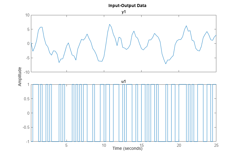
It is good practice to use only a portion of the data for estimation purposes, ze and save another part to validate the estimated models later on:
ze = z(1:200);
zv = z(201:350);
Performing Spectral Analysis
Now that we have obtained the simulated data, we can estimate models and make comparisons. Let us start with spectral analysis. We invoke the spa command which returns a spectral analysis estimate of the frequency function and the noise spectrum.
GS = spa(ze);
The result of spectral analysis is a complex-valued function of frequency: the frequency response. It is packaged into an object called IDFRD object (Identified Frequency Response Data):
GS
GS =
IDFRD model.
Contains Frequency Response Data for 1 output(s) and 1 input(s), and the spectra for disturbances at the outputs.
Response data and disturbance spectra are available at 128 frequency points, ranging from 0.09817 rad/s to 12.57 rad/s.

Sample time: 0.25 seconds
Output channels: 'y1'
Input channels: 'u1'
Status:
Estimated using SPA on time domain data "m0".

Model Properties
To plot the frequency response it is customary to use the Bode plot, with the bode or bodeplot command:
clf
h = bodeplot(GS); % bodeplot returns a plot handle, which bode does not
ax = axis;
axis([0.1 10 ax(3:4)])
The estimate GS is uncertain, since it is formed from noise corrupted data. The spectral analysis method provides also its own assessment of this uncertainty. To display the uncertainty (say for example 3 standard deviations) we can use the showConfidence command on the plot handle h returned by the previous bodeplot command.
showConfidence(h,3)

The plot says that although the nominal estimate of the frequency response (blue line) is not necessarily accurate, there is a 99.7% probability (3 standard deviations of the normal distribution) that the true response is within the shaded (light-blue) region.
Estimating Parametric State Space Models
Next let us estimate a default (without us specifying a particular model structure) linear model. It will be computed as a state-space model using a prediction error method. We use the ssest function in this case:
m = ssest(ze) % The order of the model will be chosen automaticallym =
Continuous-time identified state-space model:
dx/dt = A x(t) + B u(t) + K e(t)
y(t) = C x(t) + D u(t) + e(t)
A =
x1 x2
x1 -0.007167 1.743
x2 -2.181 -1.337
B =
u1
x1 0.09388
x2 0.2408
C =
x1 x2
y1 47.34 -14.4
D =
u1
y1 0
K =
y1
x1 0.04108
x2 -0.03751
Parameterization:
FREE form (all coefficients in A, B, C free).
Feedthrough: none
Disturbance component: estimate
Number of free coefficients: 10
Use "idssdata", "getpvec", "getcov" for parameters and their uncertainties.
Status:
Estimated using SSEST on time domain data "m0".
Fit to estimation data: 75.08% (prediction focus)
FPE: 0.9835, MSE: 0.9262
Model Properties
At this point the state-space model matrices do not tell us very much. We could compare the frequency response of the model m with that of the spectral analysis estimate GS. Note that GS is a discrete-time model while m is a continuous-time model. It is possible to use ssest to compute discrete time models too.
bodeplot(m,GS)
ax = axis;
axis([0.1 10 ax(3:4)])
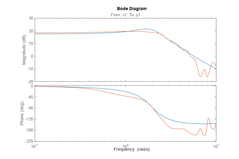
We note that the two frequency responses are close, despite the fact that they have been estimated in very different ways.
Estimating Simple Transfer Functions
There is a wide variety of linear model structures, all corresponding to linear difference or differential equations describing the relation between u and y. The different structures all correspond to various ways of modeling the noise influence. The simplest of these models are the transfer function and ARX models. A transfer function takes the form:
Y(s) = NUM(s)/DEN(s) U(s) + E(s)
where NUM(s) and DEN(s) are the numerator and denominator polynomials, and Y(s), U(s) and E(s) are the Laplace Transforms of the output, input and error signals (y(t), u(t) and e(t)) respectively. NUM and DEN can be parameterized by their orders which represent the number of zeros and poles. For a given number of poles and zeros, we can estimate a transfer function using the tfest command:
mtf = tfest(ze, 2, 2) % transfer function with 2 zeros and 2 polesmtf =
From input "u1" to output "y1":
-0.05428 s^2 - 0.02386 s + 29.6
-------------------------------
s^2 + 1.361 s + 4.102
Continuous-time identified transfer function.
Parameterization:
Number of poles: 2 Number of zeros: 2
Number of free coefficients: 5
Use "tfdata", "getpvec", "getcov" for parameters and their uncertainties.
Status:
Estimated using TFEST on time domain data "m0".
Fit to estimation data: 71.69%
FPE: 1.282, MSE: 1.195
Model Properties
AN ARX model is represented as: A(q)y(t) = B(q)u(t) + e(t),
or in long-hand,
This model is linear in coefficients. The coefficients , , ..., , , ... can be computed efficiently using a least squares estimation technique. An estimate of an ARX model with a prescribed structure - two poles, one zero and a single lag on the input is obtained as ([na nb nk] = [2 2 1]):
mx = arx(ze,[2 2 1])
mx =
Discrete-time ARX model: A(z)y(t) = B(z)u(t) + e(t)
  A(z) = 1 - 1.32 z^-1 + 0.5393 z^-2

  B(z) = 0.9817 z^-1 + 0.4049 z^-2

Sample time: 0.25 seconds

Parameterization:
   Polynomial orders:   na=2   nb=2   nk=1
   Number of free coefficients: 4
   Use "polydata", "getpvec", "getcov" for parameters and their uncertainties.

Status:
Estimated using ARX on time domain data "m0".
Fit to estimation data: 68.18% (prediction focus)
FPE: 1.603, MSE: 1.509

Model Properties
Comparing the Performance of Estimated Models
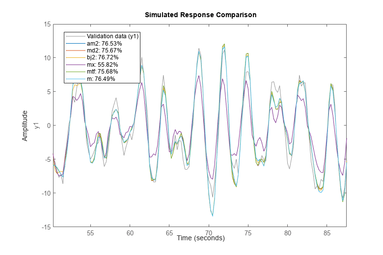
Are the models (mtf, mx) better or worse than the default state-space model m? One way to find out is to simulate each model (noise free) with the input from the validation data zv and compare the corresponding simulated outputs with the measured output in the set zv:
compare(zv,m,mtf,mx)
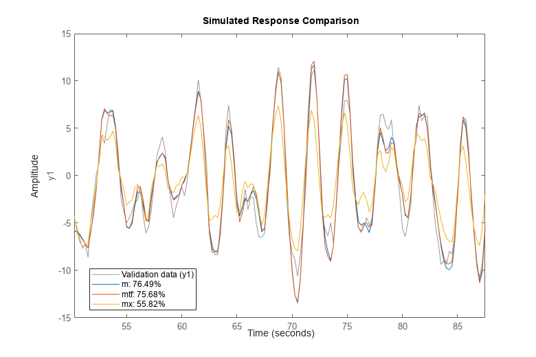
The fit is the percent of the output variation that is explained by the model. Clearly m is the better model, although mtf comes close. A discrete-time transfer function can be estimate using either the tfest or the oe command. The former creates an IDTF model while the latter creates an IDPOLY model of Output-Error structure (y(t) = B(q)/F(q)u(t) + e(t)), but they are mathematically equivalent.
md1 = tfest(ze,2,2,'Ts',0.25) % two poles and 2 zeros (counted as roots of polynomials in z^-1)
md1 =

  From input "u1" to output "y1":
   0.8383 z^-1 + 0.7199 z^-2
  ----------------------------
  1 - 1.497 z^-1 + 0.7099 z^-2

Sample time: 0.25 seconds
Discrete-time identified transfer function.

Parameterization:
   Number of poles: 2   Number of zeros: 2
   Number of free coefficients: 4
   Use "tfdata", "getpvec", "getcov" for parameters and their uncertainties.

Status:
Estimated using TFEST on time domain data "m0".
Fit to estimation data: 71.46%
FPE: 1.264, MSE: 1.214

Model Properties
md2 = oe(ze,[2 2 1])
md2 =
Discrete-time OE model: y(t) = [B(z)/F(z)]u(t) + e(t)
  B(z) = 0.8383 z^-1 + 0.7199 z^-2

  F(z) = 1 - 1.497 z^-1 + 0.7099 z^-2

Sample time: 0.25 seconds

Parameterization:
   Polynomial orders:   nb=2   nf=2   nk=1
   Number of free coefficients: 4
   Use "polydata", "getpvec", "getcov" for parameters and their uncertainties.

Status:
Estimated using OE on time domain data "m0".
Fit to estimation data: 71.46%
FPE: 1.264, MSE: 1.214

Model Properties
compare(zv, md1, md2)

The models md1 and md2 deliver identical fits to the data.
Residual Analysis
A further way to gain insight into the quality of a model is to compute the "residuals": i.e. that part e in y = Gu + He that could not be explained by the model. Ideally, these should be uncorrelated with the input and also mutually uncorrelated. The residuals are computed and their correlation properties are displayed by the resid command. This function can be used to evaluate the residues both in the time and frequency domains. First let us obtain the residuals for the Output-Error model in the time domain:
resid(zv,md2) % plots the result of residual analysis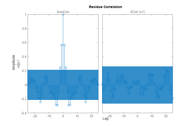
We see that the cross correlation between residuals and input lies in the confidence region, indicating that there is no significant correlation. The estimate of the dynamics G should then be considered as adequate. However, the (auto) correlation of e is significant, so e cannot be seen as white noise. This means that the noise model H is not adequate.
Estimating ARMAX and Box-Jenkins Models
Let us now compute a second order ARMAX model and a second order Box-Jenkins model. The ARMAX model has the same noise characteristics as the simulated model m0 and the Box-Jenkins model allows a more general noise description.
am2 = armax(ze,[2 2 2 1]) % 2nd order ARMAX modelam2 =
Discrete-time ARMAX model: A(z)y(t) = B(z)u(t) + C(z)e(t)
A(z) = 1 - 1.516 z^-1 + 0.7145 z^-2
B(z) = 0.982 z^-1 + 0.5091 z^-2
C(z) = 1 - 0.9762 z^-1 + 0.218 z^-2
Sample time: 0.25 seconds
Parameterization:
Polynomial orders: na=2 nb=2 nc=2 nk=1
Number of free coefficients: 6
Use "polydata", "getpvec", "getcov" for parameters and their uncertainties.
Status:
Estimated using ARMAX on time domain data "m0".
Fit to estimation data: 75.08% (prediction focus)
FPE: 0.9837, MSE: 0.9264
Model Properties
bj2 = bj(ze,[2 2 2 2 1]) % 2nd order BOX-JENKINS modelbj2 =
Discrete-time BJ model: y(t) = [B(z)/F(z)]u(t) + [C(z)/D(z)]e(t)
B(z) = 0.9922 z^-1 + 0.4701 z^-2
C(z) = 1 - 0.6283 z^-1 - 0.1221 z^-2
D(z) = 1 - 1.221 z^-1 + 0.3798 z^-2
F(z) = 1 - 1.522 z^-1 + 0.7243 z^-2
Sample time: 0.25 seconds
Parameterization:
Polynomial orders: nb=2 nc=2 nd=2 nf=2 nk=1
Number of free coefficients: 8
Use "polydata", "getpvec", "getcov" for parameters and their uncertainties.
Status:
Estimated using BJ on time domain data "m0".
Fit to estimation data: 75.47% (prediction focus)
FPE: 0.9722, MSE: 0.8974
Model Properties
Comparing Estimated Models - Simulation and Prediction Behavior
Now that we have estimated so many different models, let us make some model comparisons. This can be done by comparing the simulated outputs as before:
clf
compare(zv,am2,md2,bj2,mx,mtf,m)
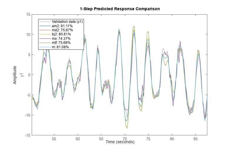
We can also compare how well the various estimated models are able to predict the output, say, 1 step ahead:
compare(zv,am2,md2,bj2,mx,mtf,m,1)
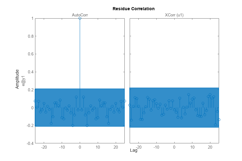
The residual analysis of model bj2 shows that the prediction error is devoid of any information - it is not auto-correlated and also uncorrelated with the input. This shows that the extra dynamic elements of a Box-Jenkins model (the C and D polynomials) were able to capture the noise dynamics.
resid(zv,bj2)
Comparing Frequency Functions
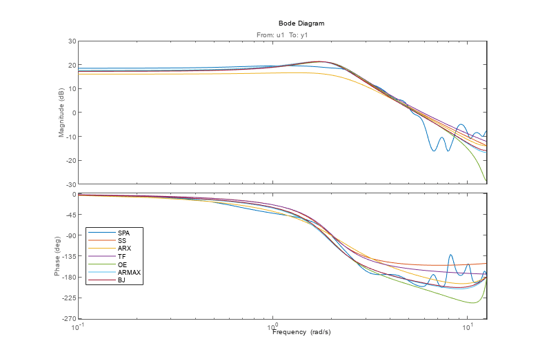
In order to compare the frequency functions for the generated models we use again the bodeplot command:
clf
w = linspace(0.1,4*pi,100);
bp = bodeplot(GS,m,mx,mtf,md2,am2,bj2,w);
bp.PhaseMatchingEnabled = 'on';
legend({'SPA','SS','ARX','TF','OE','ARMAX','BJ'},'Location','West');
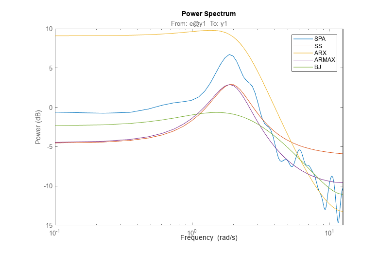
The noise spectra of the estimated models can also be analyzed. For example here we compare the noise spectra the ARMAX and the Box-Jenkins models with the state-space and the Spectral Analysis models. For this, we use the spectrum command:
spectrum(GS,m,mx,am2,bj2,w)
legend('SPA','SS','ARX','ARMAX','BJ');
Comparing Estimated Models with the True System
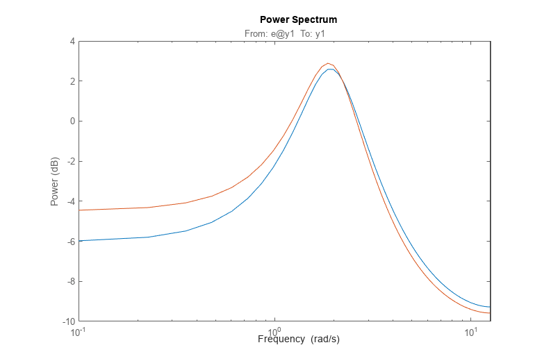
Here we validate the estimated models against the true system m0 that we used to simulate the input and output data. Let us compare the frequency functions of the ARMAX model with the true system.
bode(m0,am2,w)

The responses practically coincide. The noise spectra can also be compared.
spectrum(m0,am2,w)
Let us also examine the pole-zero plot:
h = iopzplot(m0,am2);
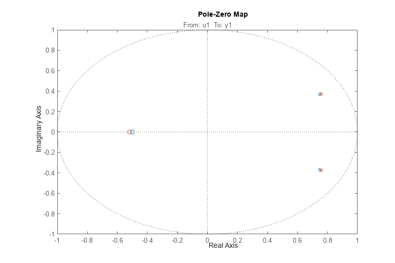
It can be seen that the poles and the zeros of the true system (blue) and the ARMAX model (green) are very close.
We can also evaluate the uncertainty of the zeros and poles. To plot confidence regions around the estimated poles and zeros corresponding to 3 standard deviations, use showConfidence or turn on the "Confidence Region" characteristic from the plot's context (right-click) menu.
showConfidence(h,3)

We see that the true, blue zeros and poles are well inside the green uncertainty regions.