Building Structured and User-Defined Models Using System Identification Toolbox

Open Script

This example shows how to estimate parameters in user-defined model structures. Such structures are specified by IDGREY (linear state-space) or IDNLGREY (nonlinear state-space) models. We shall investigate how to assign structure, fix parameters and create dependencies among them.

Experiment Data

We shall investigate data produced by a (simulated) dc-motor. We first load the data:

load dcmdata y u

The matrix y contains the two outputs: y1 is the angular position of the motor shaft and y2 is the angular velocity. There are 400 data samples and the sample time is 0.1 seconds. The input is contained in the vector u. It is the input voltage to the motor.

z = iddata(y,u,0.1); % The IDDATA object
z.InputName = 'Voltage';
z.OutputName = {'Angle';'AngVel'};
plot(z(:,1,:))

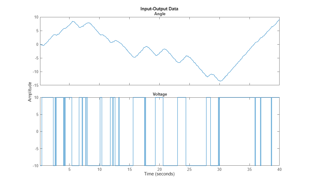
Figure: Measurement Data: Voltage to Angle

plot(z(:,2,:))

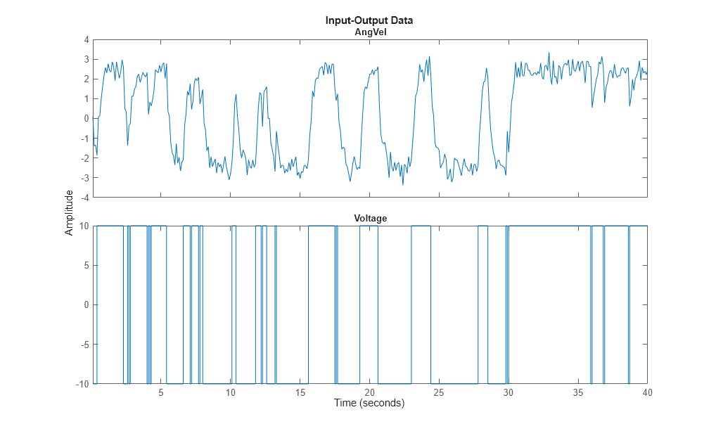
Figure: Measurement Data: Voltage to Angular Velocity

Model Structure Selection

     d/dt x = A x + B u + K e
        y   = C x + D u + e

We shall build a model of the dc-motor. The dynamics of the motor is well known. If we choose x1 as the angular position and x2 as the angular velocity it is easy to set up a state-space model of the following character neglecting disturbances: (see Example 4.1 in Ljung(1999):

         | 0     1  |      | 0   |
d/dt x = |          | x  + |     | u
         | 0   -th1 |      | th2 |

        | 1  0 |
   y =  |      | x
        | 0  1 |

The parameter th1 is here the inverse time-constant of the motor and th2 is such that th2/th1 is the static gain from input to the angular velocity. (See Ljung(1987) for how th1 and th2 relate to the physical parameters of the motor). We shall estimate these two parameters from the observed data. The model structure (parameterized state space) described above can be represented in MATLAB® using IDSS and IDGREY models. These models let you perform estimation of parameters using experimental data.

Specification of a Nominal (Initial) Model

If we guess that th1=1 and th2 = 0.28 we obtain the nominal or initial model.

A = [0 1; 0 -1]; % initial guess for A(2,2) is -1
B = [0; 0.28]; % initial guess for B(2) is 0.28
C = eye(2);
D = zeros(2,1);

Create an IDSS model object.

ms = idss(A,B,C,D);

The model is characterized by its matrices, their values, which elements are free (to be estimated) and upper and lower limits of those:

ms.Structure.a

 
ans =
 
       Name: 'A'
      Value: [2x2 double]
    Minimum: [2x2 double]
    Maximum: [2x2 double]
       Free: [2x2 logical]
      Scale: [2x2 double]
       Info: [2x2 struct]

 
1x1 param.Continuous

ms.Structure.a.Value
ms.Structure.a.Free

ans =

     0     1
     0    -1


ans =

  2x2 logical array

   1   1
   1   1

Specification of Free (Independent) Parameters Using IDSS Models

So we should now mark that it is only A(2,2) and B(2,1) that are free parameters to be estimated.

ms.Structure.a.Free = [0 0; 0 1];
ms.Structure.b.Free = [0; 1];
ms.Structure.c.Free = 0; % scalar expansion used
ms.Structure.d.Free = 0;
ms.Ts = 0;  % This defines the model to be continuous

The Initial Model

ms % Initial model

ms =
  Continuous-time identified state-space model:
      dx/dt = A x(t) + B u(t) + K e(t)
       y(t) = C x(t) + D u(t) + e(t)
 
  A = 
       x1  x2
   x1   0   1
   x2   0  -1
 
  B = 
         u1
   x1     0
   x2  0.28
 
  C = 
       x1  x2
   y1   1   0
   y2   0   1
 
  D = 
       u1
   y1   0
   y2   0
 
  K = 
       y1  y2
   x1   0   0
   x2   0   0
 
Parameterization:
   STRUCTURED form (some fixed coefficients in  A, B, C).
   Feedthrough: none
   Disturbance component: none
   Number of free coefficients: 2
   Use "idssdata", "getpvec", "getcov" for parameters and their uncertainties.

Status:                                                         
Created by direct construction or transformation. Not estimated.

Estimation of Free Parameters of the IDSS Model

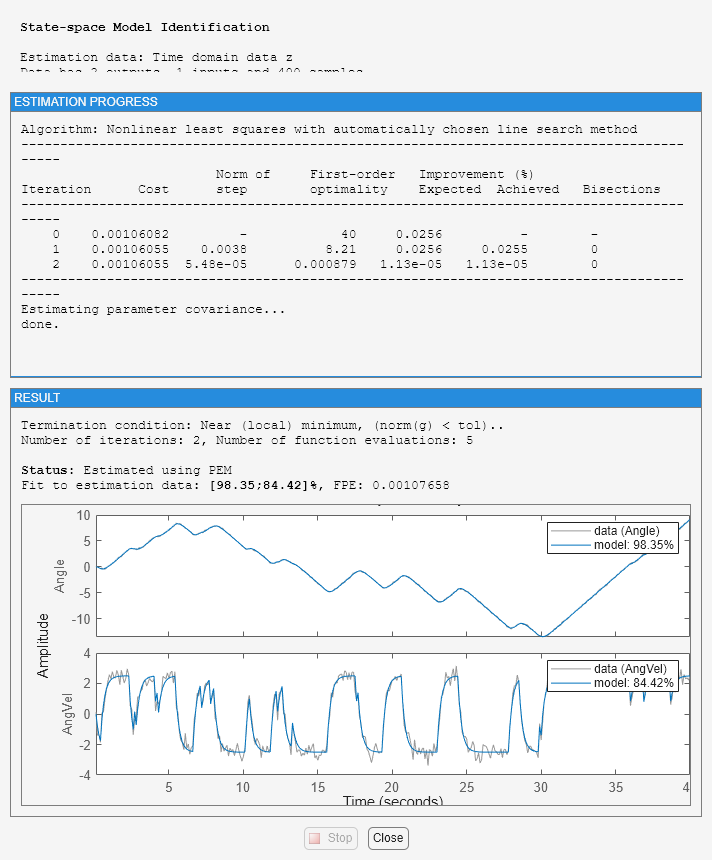
The prediction error (maximum likelihood) estimate of the parameters is now computed by:

dcmodel = ssest(z,ms,ssestOptions('Display','on'));
dcmodel

dcmodel =
  Continuous-time identified state-space model:
      dx/dt = A x(t) + B u(t) + K e(t)
       y(t) = C x(t) + D u(t) + e(t)
 
  A = 
           x1      x2
   x1       0       1
   x2       0  -4.013
 
  B = 
       Voltage
   x1        0
   x2    1.002
 
  C = 
           x1  x2
   Angle    1   0
   AngVel   0   1
 
  D = 
           Voltage
   Angle         0
   AngVel        0
 
  K = 
        Angle  AngVel
   x1       0       0
   x2       0       0
 
Parameterization:
   STRUCTURED form (some fixed coefficients in  A, B, C).
   Feedthrough: none
   Disturbance component: none
   Number of free coefficients: 2
   Use "idssdata", "getpvec", "getcov" for parameters and their uncertainties.

Status:                                       
Estimated using SSEST on time domain data "z".
Fit to estimation data: [98.35;84.42]%        
FPE: 0.001071, MSE: 0.1192

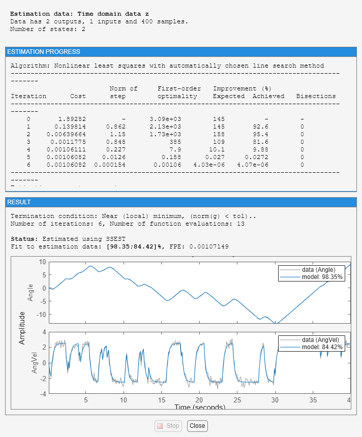
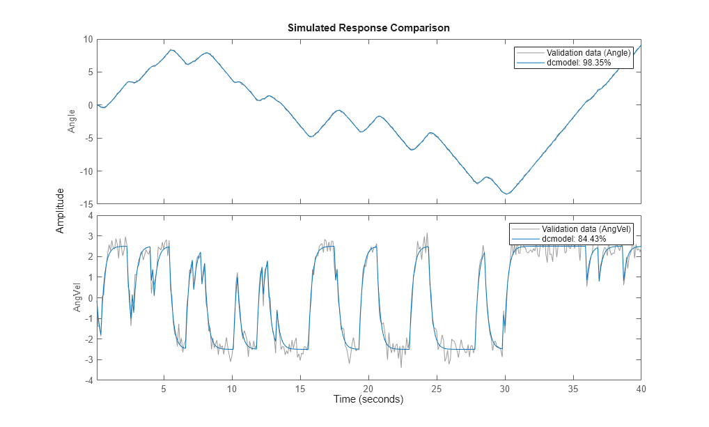
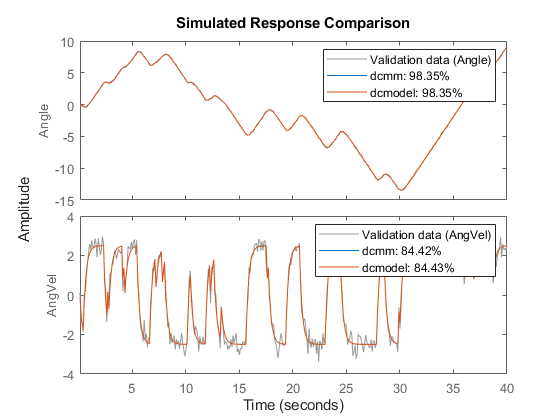
The estimated values of the parameters are quite close to those used when the data were simulated (-4 and 1). To evaluate the model's quality we can simulate the model with the actual input by and compare it with the actual output.

compare(z,dcmodel);

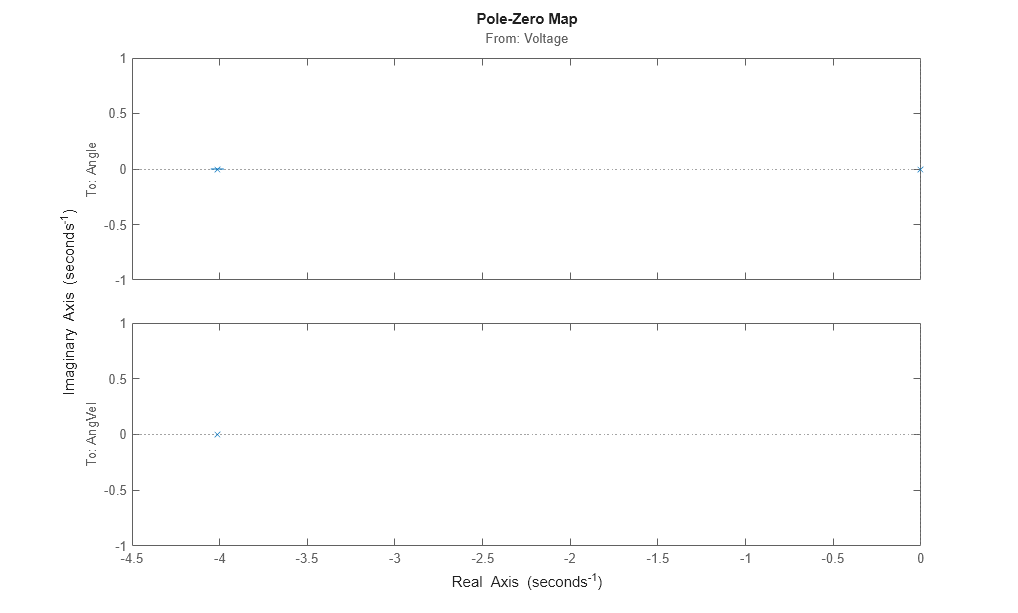
We can now, for example plot zeros and poles and their uncertainty regions. We will draw the regions corresponding to 3 standard deviations, since the model is quite accurate. Note that the pole at the origin is absolutely certain, since it is part of the model structure; the integrator from angular velocity to position.

clf
showConfidence(iopzplot(dcmodel),3)

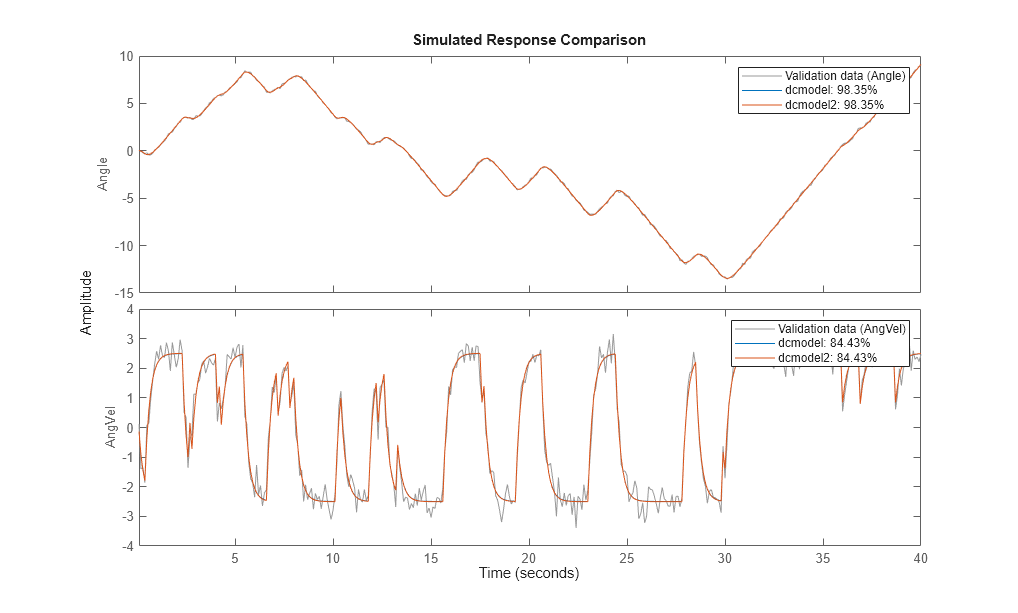
Now, we may make various modifications. The 1,2-element of the A-matrix (fixed to 1) tells us that x2 is the derivative of x1. Suppose that the sensors are not calibrated, so that there may be an unknown proportionality constant. To include the estimation of such a constant we just "let loose" A(1,2) and re-estimate:

dcmodel2 = dcmodel;
dcmodel2.Structure.a.Free(1,2) = 1;
dcmodel2 = pem(z,dcmodel2);

The resulting model is

dcmodel2

dcmodel2 =
  Continuous-time identified state-space model:
      dx/dt = A x(t) + B u(t) + K e(t)
       y(t) = C x(t) + D u(t) + e(t)
 
  A = 
           x1      x2
   x1       0  0.9975
   x2       0  -4.011
 
  B = 
       Voltage
   x1        0
   x2    1.004
 
  C = 
           x1  x2
   Angle    1   0
   AngVel   0   1
 
  D = 
           Voltage
   Angle         0
   AngVel        0
 
  K = 
        Angle  AngVel
   x1       0       0
   x2       0       0
 
Parameterization:
   STRUCTURED form (some fixed coefficients in  A, B, C).
   Feedthrough: none
   Disturbance component: none
   Number of free coefficients: 3
   Use "idssdata", "getpvec", "getcov" for parameters and their uncertainties.

Status:                                     
Estimated using PEM on time domain data "z".
Fit to estimation data: [98.35;84.42]%      
FPE: 0.001077, MSE: 0.1192

We find that the estimated A(1,2) is close to 1. To compare the two model we use the compare command:

compare(z,dcmodel,dcmodel2)

Specification of Models with Coupled Parameters Using IDGREY Objects

Suppose that we accurately know the static gain of the dc-motor (from input voltage to angular velocity, e.g. from a previous step-response experiment. If the static gain is G, and the time constant of the motor is t, then the state-space model becomes

          |0     1|    |  0  |
d/dt x =  |       |x + |     | u
          |0  -1/t|    | G/t |

          |1   0|
   y   =  |     | x
          |0   1|

With G known, there is a dependence between the entries in the different matrices. In order to describe that, the earlier used way with "Free" parameters will not be sufficient. We thus have to write a MATLAB file which produces the A, B, C, and D, and optionally also the K and X0 matrices as outputs, for each given parameter vector as input. It also takes auxiliary arguments as inputs, so that the user can change certain things in the model structure, without having to edit the file. In this case we let the known static gain G be entered as such an argument. The file that has been written has the name 'motorDynamics.m'.

type motorDynamics

function [A,B,C,D,K,X0] = motorDynamics(par,ts,aux)
%MOTORDYNAMICS ODE file representing the dynamics of a motor.
%
%   [A,B,C,D,K,X0] = motorDynamics(Tau,Ts,G)
%   returns the State Space matrices of the DC-motor with
%   time-constant Tau (Tau = par) and known static gain G. The sample
%   time is Ts.
%
%   This file returns continuous-time representation if input argument Ts
%   is zero. If Ts>0, a discrete-time representation is returned. To make
%   the IDGREY model that uses this file aware of this flexibility, set the
%   value of Structure.FcnType property to 'cd'. This flexibility is useful
%   for conversion between continuous and discrete domains required for
%   estimation and simulation.
%
%   See also IDGREY, IDDEMO7.

%   L. Ljung
%   Copyright 1986-2015 The MathWorks, Inc.

t = par(1);
G = aux(1);

A = [0 1;0 -1/t];
B = [0;G/t];
C = eye(2);
D = [0;0];
K = zeros(2);
X0 = [0;0];
if ts>0 % Sample the model with sample time Ts
   s = expm([[A B]*ts; zeros(1,3)]);
   A = s(1:2,1:2);
   B = s(1:2,3);
end

We now create an IDGREY model object corresponding to this model structure: The assumed time constant will be

par_guess = 1;

We also give the value 0.25 to the auxiliary variable G (gain) and sample time.

aux = 0.25;
dcmm = idgrey('motorDynamics',par_guess,'cd',aux,0);

The time constant is now estimated by

dcmm = greyest(z,dcmm,greyestOptions('Display','on'));

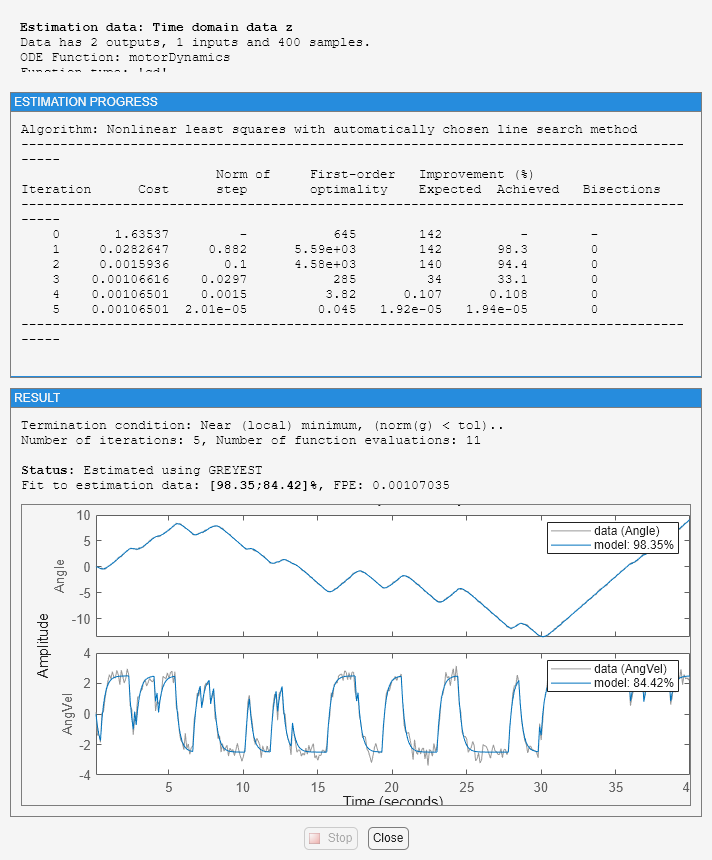
We have thus now estimated the time constant of the motor directly. Its value is in good agreement with the previous estimate.

dcmm

dcmm =
  Continuous-time linear grey box model defined by "motorDynamics" function:
      dx/dt = A x(t) + B u(t) + K e(t)
       y(t) = C x(t) + D u(t) + e(t)
 
  A = 
           x1      x2
   x1       0       1
   x2       0  -4.006
 
  B = 
       Voltage
   x1        0
   x2    1.001
 
  C = 
           x1  x2
   Angle    1   0
   AngVel   0   1
 
  D = 
           Voltage
   Angle         0
   AngVel        0
 
  K = 
        Angle  AngVel
   x1       0       0
   x2       0       0
 
  Model parameters:
   Par1 = 0.2496
 
Parameterization:
   ODE Function: motorDynamics
   (parametrizes both continuous- and discrete-time equations)
   Disturbance component: parameterized by the ODE function
   Initial state: parameterized by the ODE function
   Number of free coefficients: 1
   Use "getpvec", "getcov" for parameters and their uncertainties.

Status:                                         
Estimated using GREYEST on time domain data "z".
Fit to estimation data: [98.35;84.42]%          
FPE: 0.00107, MSE: 0.1193

With this model we can now proceed to test various aspects as before. The syntax of all the commands is identical to the previous case. For example, we can compare the idgrey model with the other state-space model:

compare(z,dcmm,dcmodel)

They are clearly very close.

Estimating Multivariate ARX Models

The state-space part of the toolbox also handles multivariate (several outputs) ARX models. By a multivariate ARX-model we mean the following:

A(q) y(t) = B(q) u(t) + e(t)

Here A(q) is a ny | ny matrix whose entries are polynomials in the delay operator 1/q. The k-l element is denoted by:

$a_{kl}(q)$

where:

$a_{kl}(q) = 1 + a_1 q^{-1} + .... + a_{nakl} q^{-nakl} q$

It is thus a polynomial in 1/q of degree nakl.

Similarly B(q) is a ny | nu matrix, whose kj-element is:

$b_{kj}(q) = b_0 q^{-nkk}+b_1 q^{-nkkj-1}+ ... +b_{nbkj} q^{-nkkj-nbkj}$

There is thus a delay of nkkj from input number j to output number k. The most common way to create those would be to use the ARX-command. The orders are specified as: nn = [na nb nk] with na being a ny-by-ny matrix whose kj-entry is nakj; nb and nk are defined similarly.

Let's test some ARX-models on the dc-data. First we could simply build a general second order model:

dcarx1 = arx(z,'na',[2,2;2,2],'nb',[2;2],'nk',[1;1])

dcarx1 =
Discrete-time ARX model:                                                   
  Model for output "Angle": A(z)y_1(t) = - A_i(z)y_i(t) + B(z)u(t) + e_1(t)
    A(z) = 1 - 0.5545 z^-1 - 0.4454 z^-2                                   
                                                                           
    A_2(z) = -0.03548 z^-1 - 0.06405 z^-2                                  
                                                                           
    B(z) = 0.004243 z^-1 + 0.006589 z^-2                                   
                                                                           
  Model for output "AngVel": A(z)y_2(t) = - A_i(z)y_i(t) + B(z)u(t) + e_2(t)
    A(z) = 1 - 0.2005 z^-1 - 0.2924 z^-2                                    
                                                                            
    A_1(z) = 0.01849 z^-1 - 0.01937 z^-2                                    
                                                                            
    B(z) = 0.08642 z^-1 + 0.03877 z^-2                                      
                                                                            
Sample time: 0.1 seconds
  
Parameterization:
   Polynomial orders:   na=[2 2;2 2]   nb=[2;2]   nk=[1;1]
   Number of free coefficients: 12
   Use "polydata", "getpvec", "getcov" for parameters and their uncertainties.

Status:                                                  
Estimated using ARX on time domain data "z".             
Fit to estimation data: [97.87;83.44]% (prediction focus)
FPE: 0.002157, MSE: 0.1398

The result, dcarx1, is stored as an IDPOLY model, and all previous commands apply. We could for example explicitly list the ARX-polynomials by:

dcarx1.a

ans =

  2x2 cell array

    {[1 -0.5545 -0.4454]}    {[0 -0.0355 -0.0640]}
    {[ 0 0.0185 -0.0194]}    {[1 -0.2005 -0.2924]}

as cell arrays where e.g. the {1,2} element of dcarx1.a is the polynomial A(1,2) described earlier, relating y2 to y1.

We could also test a structure, where we know that y1 is obtained by filtering y2 through a first order filter. (The angle is the integral of the angular velocity). We could then also postulate a first order dynamics from input to output number 2:

na = [1 1; 0 1];
nb = [0 ; 1];
nk = [1 ; 1];
dcarx2 = arx(z,[na nb nk])

dcarx2 =
Discrete-time ARX model:                                                   
  Model for output "Angle": A(z)y_1(t) = - A_i(z)y_i(t) + B(z)u(t) + e_1(t)
    A(z) = 1 - 0.9992 z^-1                                                 
                                                                           
    A_2(z) = -0.09595 z^-1                                                 
                                                                           
    B(z) = 0                                                               
                                                                           
  Model for output "AngVel": A(z)y_2(t) = B(z)u(t) + e_2(t)
    A(z) = 1 - 0.6254 z^-1                                 
                                                           
    B(z) = 0.08973 z^-1                                    
                                                           
Sample time: 0.1 seconds
  
Parameterization:
   Polynomial orders:   na=[1 1;0 1]   nb=[0;1]   nk=[1;1]
   Number of free coefficients: 4
   Use "polydata", "getpvec", "getcov" for parameters and their uncertainties.

Status:                                                  
Estimated using ARX on time domain data "z".             
Fit to estimation data: [97.52;81.46]% (prediction focus)
FPE: 0.003452, MSE: 0.177

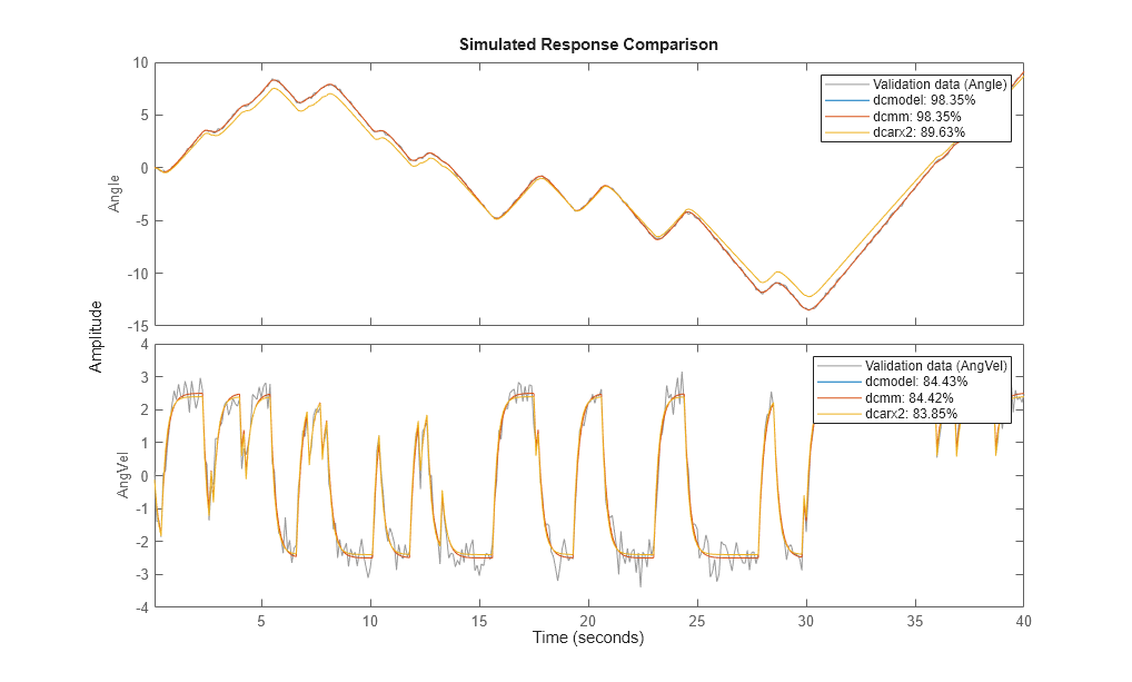
To compare the different models obtained we use

compare(z,dcmodel,dcmm,dcarx2)

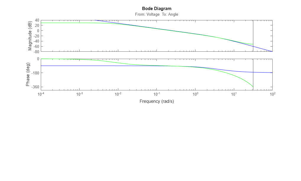
Finally, we could compare the bodeplots obtained from the input to output one for the different models by using bode: First output:

dcmm2 = idss(dcmm); % convert to IDSS for subreferencing
bode(dcmodel(1,1),'r',dcmm2(1,1),'b',dcarx2(1,1),'g')

Second output:

bode(dcmodel(2,1),'r',dcmm2(2,1),'b',dcarx2(2,1),'g')

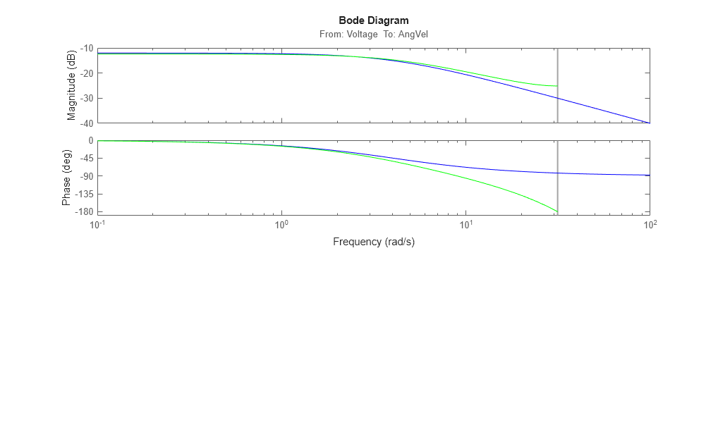
The two first models are more or less in exact agreement. The ARX-models are not so good, due to the bias caused by the non-white equation error noise. (We had white measurement noise in the simulations).

Conclusions

Estimation of models with pre-selected structures can be performed using System Identification toolbox. In state-space form, parameters may be fixed to their known values or constrained to lie within a prescribed range. If relationship between parameters or other constraints need to be specified, IDGREY objects may be used. IDGREY models evaluate a user-specified MATLAB file for estimating state-space system parameters. Multi-variate ARX models offer another option for quickly estimating multi-output models with user-specified structure.