Code Generation for a Sequence-to-Sequence Classification Using 1-D Convolutions

Since R2024a

This example shows how to generate CUDA code for a temporal convolutional network (TCN). You could also generate C code by using a CPU coder configuration instead of a GPU coder configuration. The example generates a MEX application that makes predictions at each step of an input time series. This example uses accelerometer sensor data from a smartphone carried on the body and makes predictions on the activity of the wearer. User movements are classified into one of five categories, namely dancing, running, sitting, standing, and walking. For more information of the pretrained TCN used in the example, see the Sequence-to-Sequence Classification Using 1-D Convolutions (Deep Learning Toolbox).

Third-Party Prerequisites

This example generates CUDA MEX and has the following third-party requirements.

• CUDA-enabled NVIDIA® GPU and compatible driver.

For non-MEX builds such as static, dynamic libraries or executables, this example has the following additional requirements.

• NVIDIA toolkit.

• Environment variables for the compilers and libraries. For more information, see Third-Party Hardware and Setting Up the Prerequisite Products.

Verify GPU Environment

Use the coder.checkGpuInstall function to verify that the compilers and libraries necessary for running this example are set up correctly.

envCfg = coder.gpuEnvConfig('host');
envCfg.Quiet = 1;
coder.checkGpuInstall(envCfg);

The human_activity_predict Entry-Point Function

A sequence-to-sequence 1-D CNN network allows you to make different predictions for each individual time step of a data sequence. The human_activity_predict.m entry-point function takes an input sequence and passes it to a trained TCN for prediction. The entry-point function loads the dlnetwork object from the HumanActivityNet.mat file into a persistent variable and reuses the persistent object on subsequent prediction calls. A dlarray object is created within the entry-point function. The input and output of the function are numeric data types. For more information, see Code Generation for dlarray.

type('human_activity_predict.m')

function out = human_activity_predict(net, in) %#codegen
% Copyright 2024 The MathWorks, Inc.

% The input contains two dimensions corresponding to channel and time. 
% Therefore, the dataformat passed to dlarray constructor is specified as 'CT'.
dlIn = dlarray(in,'CT');
persistent dlnet;

if isempty(dlnet)
    dlnet = coder.loadDeepLearningNetwork(net);
end

dlOut = predict(dlnet,dlIn);

out = extractdata(dlOut);
end

The main building block of a TCN is a dilated causal convolution layer, which operates over the time steps of each sequence. For more details about the network Sequence-to-Sequence Classification Using 1-D Convolutions (Deep Learning Toolbox).

netStruct = load('HumanActivityNet.mat');
disp(netStruct.net.Layers);

  36×1 Layer array with layers:

     1   'input'           Sequence Input        Sequence input with 3 dimensions
     2   'conv1_1'         1-D Convolution       64 5×3 convolutions with stride 1 and padding 'causal'
     3   'layernorm_1'     Layer Normalization   Layer normalization with 64 channels
     4   'SpatialDrop01'   Spatial Dropout       Spatial Dropout
     5   'conv1d'          1-D Convolution       64 5×64 convolutions with stride 1 and padding 'causal'
     6   'layernorm_2'     Layer Normalization   Layer normalization with 64 channels
     7   'relu'            ReLU                  ReLU
     8   'SpatialDrop02'   Spatial Dropout       Spatial Dropout
     9   'add_1'           Addition              Element-wise addition of 2 inputs
    10   'convSkip'        1-D Convolution       64 1×3 convolutions with stride 1 and padding [0  0]
    11   'conv1_2'         1-D Convolution       64 5×64 convolutions with stride 1, dilation factor 2, and padding 'causal'
    12   'layernorm_3'     Layer Normalization   Layer normalization with 64 channels
    13   'SpatialDrop21'   Spatial Dropout       Spatial Dropout
    14   'conv1d_1'        1-D Convolution       64 5×64 convolutions with stride 1, dilation factor 2, and padding 'causal'
    15   'layernorm_4'     Layer Normalization   Layer normalization with 64 channels
    16   'relu_1'          ReLU                  ReLU
    17   'SpatialDrop22'   Spatial Dropout       Spatial Dropout
    18   'add_2'           Addition              Element-wise addition of 2 inputs
    19   'conv1_3'         1-D Convolution       64 5×64 convolutions with stride 1, dilation factor 4, and padding 'causal'
    20   'layernorm_5'     Layer Normalization   Layer normalization with 64 channels
    21   'SpatialDrop41'   Spatial Dropout       Spatial Dropout
    22   'conv1d_2'        1-D Convolution       64 5×64 convolutions with stride 1, dilation factor 4, and padding 'causal'
    23   'layernorm_6'     Layer Normalization   Layer normalization with 64 channels
    24   'relu_2'          ReLU                  ReLU
    25   'SpatialDrop42'   Spatial Dropout       Spatial Dropout
    26   'add_3'           Addition              Element-wise addition of 2 inputs
    27   'conv1_4'         1-D Convolution       64 5×64 convolutions with stride 1, dilation factor 8, and padding 'causal'
    28   'layernorm_7'     Layer Normalization   Layer normalization with 64 channels
    29   'SpatialDrop61'   Spatial Dropout       Spatial Dropout
    30   'conv1d_3'        1-D Convolution       64 5×64 convolutions with stride 1, dilation factor 8, and padding 'causal'
    31   'layernorm_8'     Layer Normalization   Layer normalization with 64 channels
    32   'relu_3'          ReLU                  ReLU
    33   'SpatialDrop62'   Spatial Dropout       Spatial Dropout
    34   'add_4'           Addition              Element-wise addition of 2 inputs
    35   'fc'              Fully Connected       5 fully connected layer
    36   'softmax'         Softmax               softmax

You can also use the analyzeNetwork (Deep Learning Toolbox) function to display an interactive visualization of the network architecture and information about the network layers.

Generate CUDA MEX

To generate CUDA MEX for the human_activity_predict.m entry-point function, create a GPU configuration object and specify the target to be MEX. Create a deep learning configuration object that specifies the target library as none. Attach this deep learning configuration object to the GPU configuration object. The TCN network has 1-D convolutional layers that are only supported for code generation when TargetLibrary is set to 'none'.

cfg = coder.gpuConfig('mex');
cfg.DeepLearningConfig = coder.DeepLearningConfig(TargetLibrary='none');

At compile time, GPU Coder™ must know the data types of all the inputs to the entry-point function. Specify the input to the network for code generation.

s = load("HumanActivityData.mat");
XTest = s.XTest;
YTest = s.YTest;

Run the codegen command.

codegen -config cfg human_activity_predict -args {coder.Constant('HumanActivityNet.mat'), single(XTest{1})} -report

Code generation successful: View report

Run Generated MEX on Test Data

The HumanActivityValidate MAT-file stores the variable XTest that contains sample time series of sensor readings on which you can test the generated code. Load the MAT-file and cast the data to single for deployment. Call the human_activity_predict_mex function on the first observation.

YPred = human_activity_predict_mex('HumanActivityNet.mat',single(XTest{1}));

YPred is a 5-by-53888 numeric matrix containing the probabilities of the five classes for each of the 53888 time steps. For each time step, find the predicted class by calculating the index of the maximum probability.

[~, maxIndex] = max(YPred, [], 1);

Associate the indices of max probability to the corresponding label. Display the first ten labels. From the results, you can see that the network predicted the human to be sitting for the first ten time steps.

labels = categorical({'Dancing', 'Running', 'Sitting', 'Standing', 'Walking'});
predictedLabels1 = labels(maxIndex);
disp(predictedLabels1(1:10)')

     Sitting 
     Sitting 
     Sitting 
     Sitting 
     Sitting 
     Sitting 
     Sitting 
     Sitting 
     Sitting 
     Sitting 

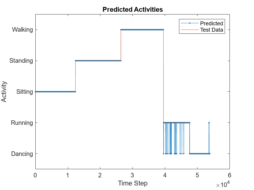
Compare Predictions with Test Data

Use a plot to compare the MEX output with the test data.

figure
plot(predictedLabels1,'.-');
hold on
plot(YTest{1});
hold off

xlabel("Time Step")
ylabel("Activity")
title("Predicted Activities")
legend(["Predicted" "Test Data"])

Copyright 2024 The MathWorks, Inc.