Pareto-Front für multiobjektive Optimierung, problembasiert
R2024aDieses Beispiel zeigt, wie ein mehrzieliges Optimierungsproblem mithilfe von Optimierungsvariablen gelöst und die Lösung grafisch dargestellt wird.
Problemformulierung
Das Problem hat eine zweidimensionale Optimierungsvariable und zwei Zielfunktionen. Erstellen Sie die Optimierungsvariable x als Zeilenvektor, die Ausrichtung wird von Mehrziellösern erwartet. Legen Sie Grenzen fest, die angeben, dass die Komponenten von x zwischen –50 und 50 liegen.
x = optimvar("x",1,2,LowerBound=-50,UpperBound=50);Erstellen Sie die zweikomponentige Zielfunktion. Integrieren Sie die Zielfunktion in ein Optimierungsproblem.
fun(1) = x(1)^4 + x(2)^4 + x(1)*x(2) - x(1)^2*x(2)^2 - 9*x(1)^2;
fun(2) = x(1)^4 + x(2)^4 + x(1)*x(2) - x(1)^2*x(2)^2 + 3*x(2)^3;
prob = optimproblem("Objective",fun);
Überprüfen Sie das Problem.
show(prob)
  OptimizationProblem :

	Solve for:
       x

	minimize :
       ((((x(1).^4 + x(2).^4) + (x(1) .* x(2))) - (x(1).^2 .* x(2).^2)) - (9 .* x(1).^2))
       ((((x(1).^4 + x(2).^4) + (x(1) .* x(2))) - (x(1).^2 .* x(2).^2)) + (3 .* x(2).^3))


	variable bounds:
       -50 <= x(1) <= 50
       -50 <= x(2) <= 50
Lösung lösen und darstellen
Rufen Sie solve an, um das Problem zu lösen.
rng default % For reproducibility
sol = solve(prob)
Solving problem using gamultiobj.
gamultiobj stopped because the average change in the spread of Pareto solutions is less than options.FunctionTolerance.
sol =
  1x18 OptimizationValues vector with properties:

   Variables properties:
            x: [2x18 double]

   Objective properties:
    Objective: [2x18 double]
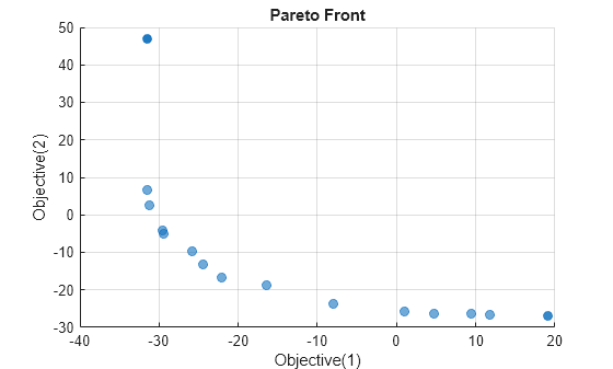
Zeichnen Sie die resultierende Pareto-Front.
paretoplot(sol)
Lösen Sie das Problem erneut mit dem paretosearch-Solver.
sol2 = solve(prob,Solver="paretosearch");Solving problem using paretosearch. Pareto set found that satisfies the constraints. Optimization completed because the relative change in the volume of the Pareto set is less than 'options.ParetoSetChangeTolerance' and constraints are satisfied to within 'options.ConstraintTolerance'.
paretoplot(sol2)
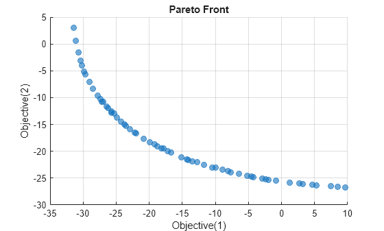
Mit den Standardoptionen erhält der paretosearch-Solver einen dichteren Satz von Lösungspunkten als gamultiobj. Allerdings erhält gamultiobj einen größeren Wertebereich.
Beginnen Sie mit Lösungen mit einem einzigen Ziel
Um eine bessere Verteilung der Lösungen zu erreichen, suchen Sie die Einzelziellösungen beginnend bei x = [1 1].
x0.x = [1 1];
prob1 = optimproblem("Objective",fun(1));
solp1 = solve(prob1,x0);
Solving problem using fmincon. Local minimum possible. Constraints satisfied. fmincon stopped because the size of the current step is less than the value of the step size tolerance and constraints are satisfied to within the value of the constraint tolerance.
prob2 = optimproblem("Objective",fun(2));
solp2 = solve(prob2,x0);
Solving problem using fmincon. Local minimum found that satisfies the constraints. Optimization completed because the objective function is non-decreasing in feasible directions, to within the value of the optimality tolerance, and constraints are satisfied to within the value of the constraint tolerance.
Bereiten Sie die Einzelziellösungen als Ausgangspunkt für solve vor. Jeder Punkt muss als Spaltenvektor an die Funktion optimvalues übergeben werden.
start = optimvalues(prob,"x",[solp1.x' solp2.x']);Lösen Sie das Mehrzielproblem mit paretosearch, ausgehend von den start-Punkten.
sol3 = solve(prob,start,Solver="paretosearch");Solving problem using paretosearch. Pareto set found that satisfies the constraints. Optimization completed because the relative change in the volume of the Pareto set is less than 'options.ParetoSetChangeTolerance' and constraints are satisfied to within 'options.ConstraintTolerance'.
paretoplot(sol3)
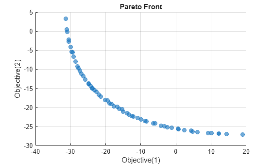
Dieses Mal findet paretosearch einen größeren Bereich der Zielfunktionen, der bei Ziel 2 fast bis 10 und bei Ziel 1 fast bis 20 geht. Dieser Bereich ähnelt dem gamultiobj-Bereich, mit Ausnahme des anomalen Lösungspunkts in der Nähe von Ziel 1 = –31, Ziel 2 = 48.
Siehe auch
gamultiobj | paretosearch | solve | paretoplot

