Fuzzy PID Control with Type-2 FIS
This example compares a type-2 fuzzy PID controller with both a type-1 fuzzy PID controller and conventional PID controller. This example is adapted from [1].
Fuzzy PID Control
This example uses the following fuzzy logic controller (FLC) structure as described in [1]. The controller is implemented using the Fuzzy PID Controller block. The output of the controller () is found using the error () and the derivative of the error (). Using scaling factors and , inputs and are normalized to and , respectively. The normalized ranges for both inputs are in the range [-1,1]. The FLC also produces a normalized output in the range [-1,1]. Additional scaling factors and map the FLC output into .
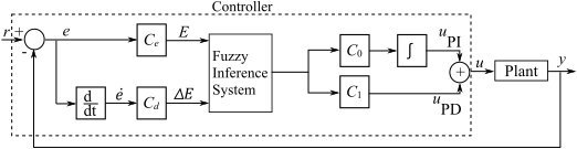
This example uses a delayed first-order system as the plant model.
Here, , , and are the gain, time delay, and time constant, respectively.
The scaling factors , , and are defined as follows, where is the closed-loop time constant.
The input scaling factor is:
where and are the reference and system output values at time . These values correspond to the nominal operating point of the system.
This example compares the performance of type-1 and type-2 Sugeno fuzzy inference systems (FISs) using the Fuzzy PID Controller block.
Construct Type-1 FIS
Create a type-1 FIS using sugfis.
fis1 = sugfis;
Add input variables to the FIS.
fis1 = addInput(fis1,[-1 1],Name="E");
fis1 = addInput(fis1,[-1 1],Name="delE");
Add three uniformly distributed overlapping triangular membership functions (MFs) to each input. The MF names stand for negative (N), zero (Z), and positive (P).
fis1 = addMF(fis1,"E","trimf",[-2 -1 0],Name="N");
fis1 = addMF(fis1,"E","trimf",[-1 0 1],Name="Z");
fis1 = addMF(fis1,"E","trimf",[0 1 2],Name="P");
fis1 = addMF(fis1,"delE","trimf",[-2 -1 0],Name="N");
fis1 = addMF(fis1,"delE","trimf",[-1 0 1],Name="Z");
fis1 = addMF(fis1,"delE","trimf",[0 1 2],Name="P");
Plot the input membership functions.
figure
subplot(1,2,1)
plotmf(fis1,"input",1)
title("Input 1")
subplot(1,2,2)
plotmf(fis1,"input",2)
title("Input 2")

Add the output variable to the FIS.
fis1 = addOutput(fis1,[-1 1],Name="U");Add uniformly distributed constant functions to the output. The MF names stand for negative big (NB), negative medium (NM), zero (Z), positive medium (PM), and positive big (PB).
fis1 = addMF(fis1,"U","constant",-1,Name="NB");
fis1 = addMF(fis1,"U","constant",-0.5,Name="NM");
fis1 = addMF(fis1,"U","constant",0,Name="Z");
fis1 = addMF(fis1,"U","constant",0.5,Name="PM");
fis1 = addMF(fis1,"U","constant",1,Name="PB");
Add rules to the FIS. These rules create a proportional control surface.
rules = [...
    "E==N & delE==N => U=NB"; ...
    "E==Z & delE==N => U=NM"; ...
    "E==P & delE==N => U=Z"; ...
    "E==N & delE==Z => U=NM"; ...
    "E==Z & delE==Z => U=Z"; ...
    "E==P & delE==Z => U=PM"; ...
    "E==N & delE==P => U=Z"; ...
    "E==Z & delE==P => U=PM"; ...
    "E==P & delE==P => U=PB" ...
    ];
fis1 = addRule(fis1,rules);
Plot the control surface.
figure
gensurf(fis1)
title("Control surface of type-1 FIS")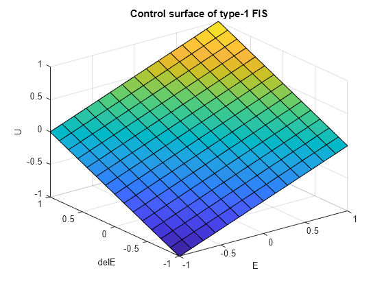
You can also load the fuzzy inference system from type1FuzzyController.fis.
fis1 = readfis("type1FuzzyController.fis");
Construct Type-2 FIS
Convert the type-1 FIS, fis1, to a type-2 FIS.
fis2 = convertToType2(fis1);
The type-2 Sugeno system, fis2, uses type-2 membership functions for the input variables and type-1 membership functions for the output variables.
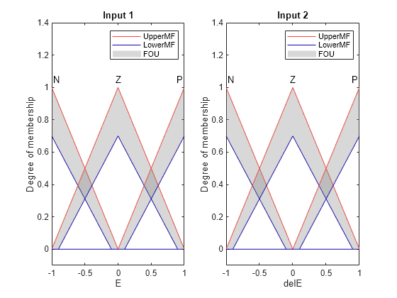
Define the footprint of uncertainty (FOU) for the input MFs as defined in [1]. To do so, set the lower MF scaling factor for each MF. For this example, set the lower MF lag values to 0.
scale = [0.2 0.9 0.2;0.3 0.9 0.3];
for i = 1:length(fis2.Inputs)
    for j = 1:length(fis2.Inputs(i).MembershipFunctions)
        fis2.Inputs(i).MembershipFunctions(j).LowerLag = 0;
        fis2.Inputs(i).MembershipFunctions(j).LowerScale = scale(i,j);
    end
end
Plot the type-2 input membership functions.
figure
subplot(1,2,1)
plotmf(fis2,"input",1)
title("Input 1")
subplot(1,2,2)
plotmf(fis2,"input",2)
title("Input 2")

You can also load the fuzzy inference system from type2FuzzyController.fis.
fis2 = readfis("type2FuzzyController.fis");
The FOU adds additional uncertainty to the FIS and produces a nonlinear control surface.
figure
gensurf(fis2)
title("Control surface of type-2 FIS")
Conventional PID Controller
This example compares the FLC performance with that of the following conventional PID controller.
Here, is proportional gain, is integrator gain, is derivative gain, and is the derivative filter time constant.
Configure Simulation
Define the nominal plant model.
C = 0.5;
L = 0.5;
T = 0.5;
G = tf(C,[T 1],Outputdelay=L);
Generate the conventional PID controller parameters using pidtune.
pidController = pidtune(G,"pidf");In this example, the reference ( is a step signal and , which results in as follows.
=1.
Ce = 1;
To configure the simulation, use the following nominal controller parameters.
tauC = 0.2;

Cd = min(T,L/2)*Ce;
C0 = 1/(C*Ce*(tauC+L/2));
C1 = max(T,L/2)*C0;
To simulate the controllers, use the comparepidcontrollers Simulink® model.
model = "comparepidcontrollers";
load_system(model)
Simulate Nominal Process
Simulate the model at the nominal operating conditions.
out1 = sim(model);
Plot the step response of the system for all three controllers.
plotOutput(out1,"Nominal",C,L,T)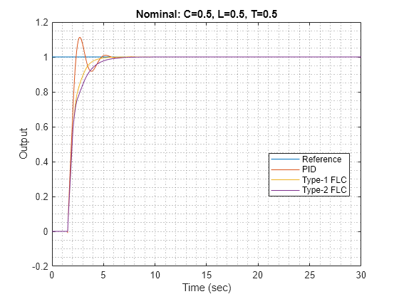
Obtain the step-response characteristics of the system for each controller. Here, rise time and settling time are in seconds, overshoot is a percentage of the final value, and the absolute error is integrated over the step response.
stepResponseTable(out1)
ans=3×4 table
                  Rise Time    Overshoot    Settling Time    Absolute Error
                  _________    _________    _____________    ______________

    PID            0.62412      11.234         4.5583              1.04
    Type-1 FLC      1.4353           0         4.1172            1.1552
    Type-2 FLC      1.8582           0         5.1278             1.279
For the nominal process:
Both the type-1 and type-2 FLCs outperform the conventional PID controller in terms of overshoot.
The conventional PID controller, performs better with respect to rise-time and integral of absolute error (IAE).
The type-1 FLC performs better than the type-2 FLC in terms of rise-time, settling-time, and IAE.
Simulate Modified Process
Modify the plant model by increasing the gain, time delay, and time constant values as compared to the nominal process.
C = 0.85;
L = 0.6;
T = 0.6;
G = tf(C,[T 1],Outputdelay=L);
Simulate the model using the updated plant parameters.
out2 = sim(model);
Plot the step response of the system for all three controllers.
plotOutput(out2,"Modified 1",C,L,T)
Obtain the step-response characteristics of the system for each controller.
stepResponseTable(out2)
ans=3×4 table
                  Rise Time    Overshoot    Settling Time    Absolute Error
                  _________    _________    _____________    ______________

    PID            0.38464      80.641         29.458            4.7486
    Type-1 FLC     0.47241      25.555         4.7309            1.1309
    Type-2 FLC     0.47209      23.958         3.4148            1.0851
For this modified process:
The conventional PID controller exhibits significant overshoot, larger settling-time, and higher IAE as compared to the FLCs.
For all performance measures, the type-2 FLC produces the same or superior performance compared to the type-1 FLC.
Conclusion
Overall, the type-1 FLC produces superior performance for the nominal plant as compared to the conventional PID controller. The type-2 FLC shows more robust performance for the modified plant.
The robustness of the conventional PID controller can be improved using different methods, such as prediction or multiple PID controller configurations. On the other hand, the performance of a type-2 FLC can be improved by using a different:
Rule base
Number of rules
FOU
For example, you can create a type-2 FLC that defines the FOU using both the lower MF scaling factor and lower MF lag.
For fis2, set the lower MF scale and lag values to 0.7 and 0.1, respectively for all input membership functions.
for i = 1:length(fis2.Inputs)
    for j = 1:length(fis2.Inputs(i).MembershipFunctions)
        fis2.Inputs(i).MembershipFunctions(j).LowerScale = 0.7;
        fis2.Inputs(i).MembershipFunctions(j).LowerLag = 0.1;
    end
end
Plot the updated membership functions.
figure
subplot(1,2,1)
plotmf(fis2,"input",1)
title("Input 1")
subplot(1,2,2)
plotmf(fis2,"input",2)
title("Input 2")
Simulate the model using the nominal plant, and plot the step responses for the controllers.
C = 0.5;
L = 0.5;
T = 0.5;
G = tf(C,[T 1],Outputdelay=L);

out4 = sim(model);
plotOutput(out4,"Nominal",C,L,T)
Obtain the step-response characteristics of the system for each controller.
stepResponseTable(out4)
ans=3×4 table
                  Rise Time    Overshoot    Settling Time    Absolute Error
                  _________    _________    _____________    ______________

    PID            0.62412      11.234         4.5583              1.04
    Type-1 FLC      1.4353           0         4.1172            1.1552
    Type-2 FLC      1.2233           0         3.9064            1.1126
In this case, the updated FOU of type-2 FLC improves the rise-time of the step response.
However, the lower MF lag values also increase the overshoot in the case of the modified plant.
C = 0.85;
L = 0.6;
T = 0.6;
G = tf(C,[T 1],Outputdelay=L);

out5 = sim(model);
plotOutput(out5,"Modified",C,L,T)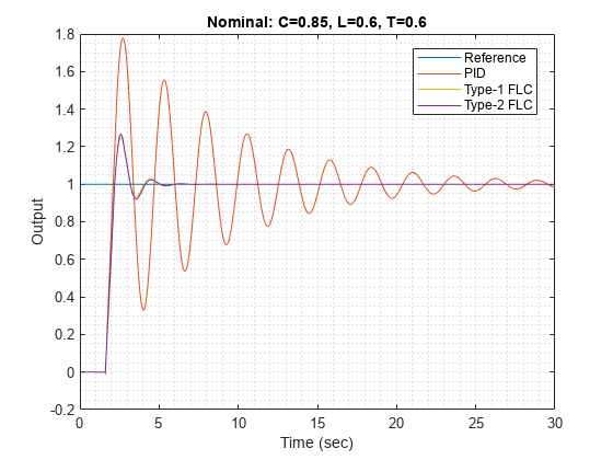
t = stepResponseTable(out5)
t=3×4 table
                  Rise Time    Overshoot    Settling Time    Absolute Error
                  _________    _________    _____________    ______________

    PID            0.38464      80.641         29.458            4.7486
    Type-1 FLC     0.47241      25.555         4.7309            1.1309
    Type-2 FLC     0.47241      27.398         4.7273            1.1427
Therefore, to obtain desired step response characteristics, you can vary the lower MF scale and lag values to find a suitable combination.
You can further improve the FLC outputs using a Mamdani type FIS since it also provides lower MF scale and lag parameters for output membership functions. However, a Mamdani type-2 FLC introduces additional computational delay due to the expensive type-reduction process.
References
[1] Mendel, J. M., Uncertain Rule-Based Fuzzy Systems: Introduction and New Directions, Second Edition, Springer, 2017, pp. 229-234, 600-608.
Local Functions
function plotOutput(out,titlePrefix,C,L,T)
figure
plot([0 20],[1 1])
hold on
plot(out.yout{1}.Values)
plot(out.yout{2}.Values)
plot(out.yout{3}.Values)
hold off
grid minor
xlabel("Time (sec)")
ylabel("Output")
title(titlePrefix + ": " + "C=" + C + ", L=" + L + ", T=" + T)
legend(["Reference","PID","Type-1 FLC","Type-2 FLC"], ...
    Location="best")
end
function t = stepResponseTable(out)
s = stepinfo(out.yout{1}.Values.Data,out.yout{1}.Values.Time);
stepResponseInfo(1).RiseTime = s.RiseTime;
stepResponseInfo(1).Overshoot = s.Overshoot;
stepResponseInfo(1).SettlingTime = s.SettlingTime;
stepResponseInfo(1).IAE = out.yout{4}.Values.Data(end);

s = stepinfo(out.yout{2}.Values.Data,out.yout{2}.Values.Time);
stepResponseInfo(2).RiseTime = s.RiseTime;
stepResponseInfo(2).Overshoot = s.Overshoot;
stepResponseInfo(2).SettlingTime = s.SettlingTime;
stepResponseInfo(2).IAE = out.yout{5}.Values.Data(end);

s = stepinfo(out.yout{3}.Values.Data,out.yout{3}.Values.Time);
stepResponseInfo(3).RiseTime = s.RiseTime;
stepResponseInfo(3).Overshoot = s.Overshoot;
stepResponseInfo(3).SettlingTime = s.SettlingTime;
stepResponseInfo(3).IAE = out.yout{6}.Values.Data(end);

t = struct2table(stepResponseInfo, ...
    RowNames=["PID" "Type-1 FLC" "Type-2 FLC"]);
t.Properties.VariableNames(1) = "Rise Time";
t.Properties.VariableNames(2) = t.Properties.VariableNames(2);
t.Properties.VariableNames(3) = "Settling Time";
t.Properties.VariableNames(4) = "Absolute Error";
end