Optimize Lookup Tables for Multiple Functions

R2026b

Since R2026b

When multiple functions in a design share input signals, you can speed up lookup table optimization for these functions by sharing breakpoints and prelookup tasks. Using multi-function lookup table optimization, you can generate optimized lookup tables from:

• Existing Lookup Table blocks

• Functions or function handles with up to three dimensions

• Simulink^® blocks including Math Function blocks, subsystems, and MATLAB Function blocks

• Curve fit and surface fit objects

Multi-function approximation is available at the command line when you specify multiple functions as inputs to a FunctionApproximation.Problem object.

Set Up a Multi-Function Approximation Problem

To create optimized lookup tables for multiple functions simultaneously, define a multi-function approximation problem. Pass a cell array of functions as the function argument when you create a FunctionApproximation.Problem object. In this example, specify the functions sin and exp.

funcs = {@(x) sin(x), @(x) exp(-x)};
problem = FunctionApproximation.Problem(funcs)

problem = 
  1×1 FunctionApproximation.Problem with properties:

    FunctionToApproximate: {[@(x)sin(x)]  [@(x)exp(-x)]}
           NumberOfInputs: 1
          NumberOfOutputs: 2
               InputTypes: "numerictype(0,16,13)"
         InputLowerBounds: 0
         InputUpperBounds: 6.2832
               OutputType: ["numerictype(1,16,14)"    "numerictype(1,16,14)"]
                  Options: [1×1 FunctionApproximation.Options]

The FunctionToApproximate property shows both functions to approximate. The problem has one input and two outputs.

These properties apply to both functions: InputLowerBounds, InputUpperBounds, and InputTypes. Adjust the shared properties.

problem.InputLowerBounds = 0;
problem.InputUpperBounds = 1.5;
problem.InputTypes = "numerictype(1,16,12)";

Each function can have a unique OutputType. To set unique output types, provide the output types as an ordered array. Each entry in the array corresponds to the function at the same position in the cell array used as the function argument.

problem.OutputType = ["numerictype(1,16,14)", "numerictype(1,16,13)"];

Configure Optimization Options

Edit the FunctionApproximation.Options object to specify constraints for the optimization. To generate MATLAB^® function files, set ApproximateSolutionType to "MATLAB".

problem.Options.WordLengths = 16;
problem.Options.BreakpointSpecification = "EvenSpacing";
problem.Options.Interpolation = "Linear";
problem.Options.ApproximateSolutionType = "MATLAB";

Settings for FunctionApproximation.Options properties apply to all input functions. These properties can have unique settings for each function:

• AbsTol

• RelTol

• OnCurveTableValues

Set per-function constraints using ordered arrays where each element corresponds to one function.

problem.Options.AbsTol = [2^-7, 2^-6];
problem.Options.RelTol = [2^-6, 2^-5];

If values that can be specified per-function are specified as a scalar value rather than as an ordered array, the value will apply to all functions.

problem.Options.OnCurveTableValues = true;

Some properties of FunctionApproximation.Options are not supported for multi-function problems. For a comprehensive list, see Multi-Function Lookup Table Optimization Limitations.

Solve the Optimization Problem

Use the solve method to find a solution that meets all per-function accuracy constraints simultaneously. The solver explores multiple candidate solutions with varying table sizes and breakpoint specifications.

sol = solve(problem)

Searching for fixed-point solutions.

|  ID | Total Memory (bits) | Feasible | Table Size | Breakpoints WLs | TableData WL | BreakpointSpecification | Normalized error (%) | 
|   0 |                  96 |        0 |          2 |              16 |      [16 16] |             EvenSpacing |           1943.1491% |
|   1 |                 352 |        1 |         10 |              16 |      [16 16] |             EvenSpacing |             22.4934% |
|   2 |                 320 |        1 |          9 |              16 |      [16 16] |             EvenSpacing |             28.3716% |
|   3 |                 288 |        1 |          8 |              16 |      [16 16] |             EvenSpacing |             37.1316% |
|   4 |                 256 |        1 |          7 |              16 |      [16 16] |             EvenSpacing |             50.3955% |
|   5 |                 224 |        1 |          6 |              16 |      [16 16] |             EvenSpacing |             72.2261% |
|   6 |                 192 |        0 |          5 |              16 |      [16 16] |             EvenSpacing |            113.6880% |
|   7 |                 160 |        0 |          4 |              16 |      [16 16] |             EvenSpacing |            200.7924% |
|   8 |                  96 |        0 |          2 |              16 |      [16 16] |         EvenPow2Spacing |           1000.9284% |
|   9 |                 160 |        0 |          4 |              16 |      [16 16] |         EvenPow2Spacing |            200.7924% |
|  10 |                 256 |        1 |          7 |              16 |      [16 16] |         EvenPow2Spacing |             50.3955% |

Best Solution
|  ID | Total Memory (bits) | Feasible | Table Size | Breakpoints WLs | TableData WL | BreakpointSpecification | Normalized error (%) |
|   5 |                 224 |        1 |          6 |              16 |      [16 16] |             EvenSpacing |             72.2261% |

sol = 
  1×1 FunctionApproximation.LUTSolution with properties:

          ID: 5
    Feasible: "true"

The search progress table in the solver displays a TableData WL column that shows an ordered vector with the word length applied to each function.

The Normalized error in the table shows the maximum of the per-function normalized error values.

Compare Solutions to Original Functions

Compare the numerical behavior of the original functions with the lookup table approximation. The comparison plot shows the approximation error for each function.

compare(sol)

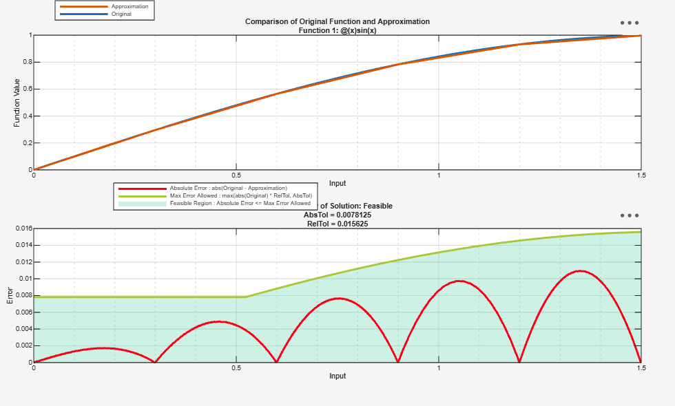
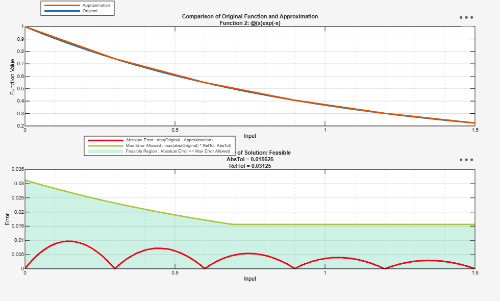
ans = struct with fields:
    Breakpoints: {[6145×1 double]}
       Original: [6145×2 double]
    Approximate: [6145×2 double]

Use the TableData structure to access the shared breakpoints and per-function table values.

t = sol.TableData

t = struct with fields:
       BreakpointValues: {[0 0.2998 0.5996 0.8994 1.1992 1.4990]}
    BreakpointDataTypes: [1×1 embedded.numerictype]
            TableValues: {[0 0.2953 0.5643 0.7830 0.9318 0.9974]  [1 0.7410 0.5491 0.4069 0.3014 0.2234]}
          TableDataType: [1×2 embedded.numerictype]
          IsEvenSpacing: 1
          Interpolation: Linear

Get the total memory usage of the optimized solution in bits. This value is the combined memory required for all shared breakpoints and table values.

sol.totalMemoryUsage

ans = 
224

Generate the Lookup Table Approximation

Use the approximate method to generate MATLAB function files containing the optimized lookup tables. Use the "Name" argument to specify output file names for each function.

approximate(sol, "Name", ["sinApprox", "expApprox"])

Multi-Function Lookup Table Optimization Limitations

The multi-function optimization workflow is available at the command line only. The Lookup Table Optimizer app does not support multiple input functions.

Subsystems with multiple outputs are not supported inputs to a multi-function FunctionApproximation.Problem..

The replaceWithApproximate and revertToOriginal methods are not supported.

These FunctionApproximation.Options properties and settings are not supported:

• AUTOSARCompliant, UseParallel, and HDLOptimized set to true.

• BreakpointSpecification property set to ExplicitValues.

• Interpolation property set to None.