Use treeviewer to Examine HWTree and PriceTree When Pricing European Callable Bond
This example demonstrates how to use treeviewer to examine tree information for a Hull-White tree when you price a European callable bond.
Specify Input Parameters
Define the interest-rate curve information.
Rates = [0.035; 0.042147; 0.047345; 0.052707];
ValuationDate = 'Jan-1-2019';
EndDates = {'Jan-1-2020'; 'Jan-1-2021'; 'Jan-1-2022'; 'Jan-1-2023'};
Compounding = 1;
Define the callable bond instruments. The first instrument is the first entry in the arrays. So, for example, the first instrument has a strike price of $98 and a maturity of January 1, 2022.
Settle = '01-Jan-2019';
Maturity = {'01-Jan-2022'; '01-Jan-2023'};
CouponRate = {{'01-Jan-2021' .0425; '01-Jan-2023' .0450}};
OptType = 'call';
Strike = [98; 95];
ExerciseDates= {'01-Jan-2021'; '01-Jan-2022'};
Basis = 1;
Define the volatility information and HW one-factor parameters.
VolDates = ['1-Jan-2020'; '1-Jan-2021'; '1-Jan-2022'; '1-Jan-2023'];
VolCurve = 0.05;
AlphaDates = '01-01-2023';
AlphaCurve = 0.05;
Build Hull-White One-Factor Tree
Use hwtree to build a one-factor tree.
RateSpec = intenvset('ValuationDate', ValuationDate, 'StartDates', ValuationDate,...
'EndDates', EndDates,'Rates', Rates, 'Compounding', Compounding, 'Basis', Basis);
HWVolSpec = hwvolspec(RateSpec.ValuationDate, VolDates, VolCurve, AlphaDates, AlphaCurve);
HWTimeSpec = hwtimespec(RateSpec.ValuationDate, VolDates, Compounding);
HWTimeSpec.Basis = Basis;

HWT = hwtree(HWVolSpec, RateSpec, HWTimeSpec);
Price Both Callable Instruments
Use optembndbyhw to price the callable bond with embedded options.
[Price, PriceTree] = optembndbyhw(HWT, CouponRate,  Settle, Maturity, OptType, Strike,...
ExerciseDates, 'Period', 1, 'Basis', Basis)
Price = 2×1

   96.4131
   92.9341
PriceTree = struct with fields:
                FinObj: 'HWPriceTree'
                  tObs: [0 1 2 3 4]
                 PTree: {[2×1 double]  [2×3 double]  [2×5 double]  [2×7 double]  [2×7 double]}
              ProbTree: {[1]  [0.1667 0.6667 0.1667]  [0.0238 0.2218 0.5087 0.2218 0.0238]  [0.0029 0.0473 0.2374 0.4247 0.2374 0.0473 0.0029]  [0.0029 0.0473 0.2374 0.4247 0.2374 0.0473 0.0029]}
                ExTree: {[2×1 double]  [2×3 double]  [2×5 double]  [2×7 double]  [2×7 double]}
            ExProbTree: {[2×1 double]  [2×3 double]  [2×5 double]  [2×7 double]  [2×7 double]}
    ExProbsByTreeLevel: [2×5 double]
               Connect: {[2]  [2 3 4]  [2 3 4 5 6]}
Examine Hull-White Tree Structure
Use treeviewer to examine the Hull-White interest-rate tree that is the input for the embedded option pricer.
treeviewer(HWT)
The Hull-White tree has 4 levels of nodes. The root node is at t = 0, three nodes are at t = 1, five nodes are at t = 2, and seven nodes are at t = 3. Each node represents a particular state. In this case, the state is defined by the forward interest-rate curve, HWT.FwdTree. The combination of HWT.FwdTree and HWT.Connect defines the tree structure. FwdTree contains the values of the forward interest rate at each node. The other fields contain other information relevant to interpreting the values in FwdTree. The most important are VolSpec, TimeSpec, and RateSpec, which contain the volatility, time structure, and rate structure information, respectively.
For example, HWT.FwdTree is:
HWT.FwdTree
ans=1×4 cell array
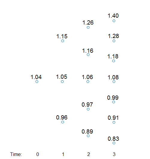
{[1.0350]} {[1.1457 1.0507 0.9635]} {[1.2639 1.1590 1.0629 0.9747 0.8938]} {[1.4003 1.2841 1.1776 1.0799 0.9903 0.9081 0.8328]}
If you display the nodes graphically with the forward rates superimposed it looks like:
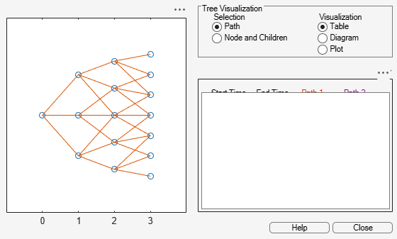
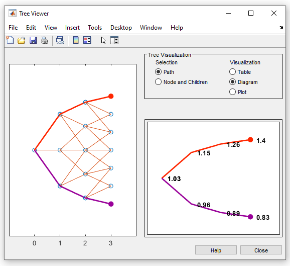
You can use the treeviewer function to visualize the rates in the tree with treeviewer(HWT). This function displays the structure of a Hull-White tree (HWT) in the left pane. The tree visualization in the right pane is blank. Visualize the actual interest-rate tree:
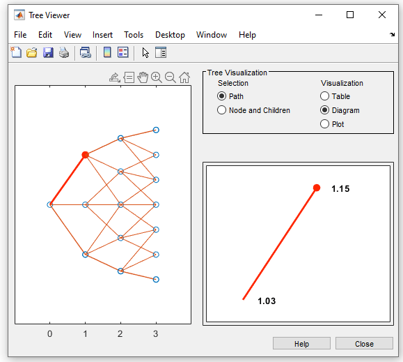
1. In the Tree Visualization pane, click Path and Diagram.
2. Select the first path by clicking the first node of the up branch at t = 1.
3. Continue by clicking the up branch at the next node at t = 2.
The following figures show the treeviewer path diagrams for these selections.
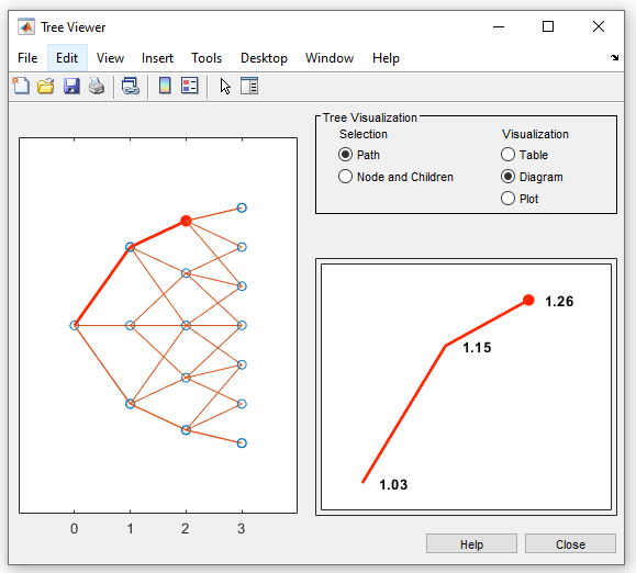
4. Continue clicking all nodes in succession until you reach the end of the branch. The entire path you selected is highlighted in red.
5. Select a second path by clicking the first node of the lower branch at t = 1. Continue clicking lower nodes as you did on the first branch. The second branch is highlighted in purple.
Hull-White trees have two additional properties called Probs and Connect. The Probs property represents the transition probabilities and the Connect property defines how the nodes are connected together.
Connect Field
HWT.Connect describes the connectivity of the nodes of a given tree level to the nodes at the next tree level.
HWT.Connect
ans=1×3 cell array
    {[2]}    {[2 3 4]}    {[2 3 4 5 6]}
The first value of HWT.Connect corresponds to t = 0 for the root node and indicates that the root node connects to node 2 of the next level at t = 1. To visualize this, consider the following connection illustration of the tree, where the node numbers have been superimposed above each node.
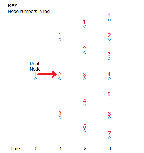
Specifically, HWT.Connect represents the index of the node in the next tree level (t + 1) that the middle branch of the node connects to.
The next entry in HWT.Connect at t = 1 is [2,3,4]. This means that node 1 at t = 1 has a middle branch with node 2 at t = 2, node 2 at t = 1 has a middle branch with node 3 at t = 2, and node 3 at t = 1 has a middle branch with node 4 at t = 2. A graphic representation follows.
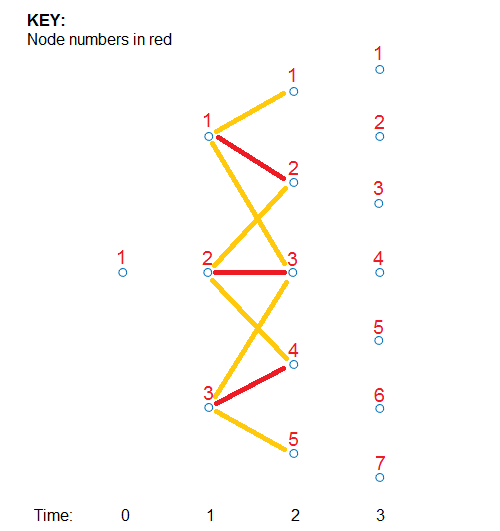
The middle branch path, as explicitly defined in HWT.Connect, is colored red and the implicit upper and lower branch paths are colored yellow. Overlaying all paths defined in HWT.Connect as red and the implicit upper and lower branches as yellow produces the following tree structure.
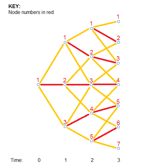
The shape in the figure is the same shape obtained by running the function treeviewer(HWT).
Probs Field
Using the following illustration, consider that you want to know the probability at t = 1 (second level of the tree) that the top node takes of one of the three paths.
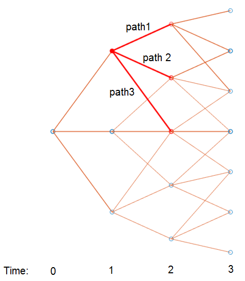
HWT.Probs gives the probabilities that a particular branch has of moving from a given node to a node on the next level of the tree.
HWT.Probs
ans=1×3 cell array
    {3×1 double}    {3×3 double}    {3×5 double}
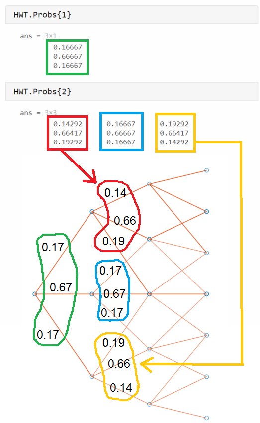
The Probs field consists of a cell array with one cell per level of the tree. Find the probabilities of all three nodes at t = 1, which corresponds to the second level of the tree.
HWT.Probs{2}ans = 3×3
0.1429 0.1667 0.1929
0.6642 0.6667 0.6642
0.1929 0.1667 0.1429
Each column represents a different node. The first node at t = 1 corresponds to the first column and the probabilities are 14.29%, 66.42%, and 19.30%.
The probability of moving up (path 1) is the top value (14.29%), the middle path is the middle value (66.42%), and the path going down (path 3) is the bottom value in the array (19.30%). The following diagram summarizes this information.
Examine the PriceTree Structure
The output of the pricing function is PriceTree. PriceTree has the following fields.
PriceTree.PTree— contains the clean prices of each instrument.PriceTree.ExTree— contains the exercise indicator arrays where a value of1indicates the option has been exercised and a value of0indicates the option has not been exercised.PriceTree.ExProbTree— contains the exercise probabilities. A value of 0 indicates there was no exercise and a nonzero value gives the probability of reaching that node where the exercise happens.PriceTree.ProbTree— contains the probability tree indicating how likely any node is reached from the root node.PriceTree.ExProbsByTreeLevel— contains the exercise probability for a given option at each tree observation time. This is an aggregated view ofPriceTree.ExProbTreethat sums the values along all nodes at a particular time.
Note that for ProbTree, PTree, ExTree, and ExProbTree, each cell represents a different time in the tree, and inside each cell is an array. Each column in the array represents a different node on the tree at that particular tree level. This structure is the same as in HWT.Probs. However, for PTree, ExTree, and ExProbTree each row represents a different instrument. Because this example prices two instruments, there are only two rows. ProbTree contains only one row as the probability of reaching a particular node is independent of the instrument being priced.
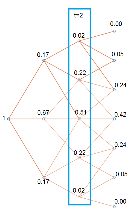
Looking at PriceTree.ProbTree, examine the probabilities of reaching each of the five nodes from the root node at t = 2, which is the third level of the tree.
PriceTree.ProbTree{3}ans = 1×5
0.0238 0.2218 0.5087 0.2218 0.0238
These results are displayed in the following diagram, where all nodes are overlayed with their probabilities. The root node at t = 0 always has a probability of being reached, hence, it has a value of 1.
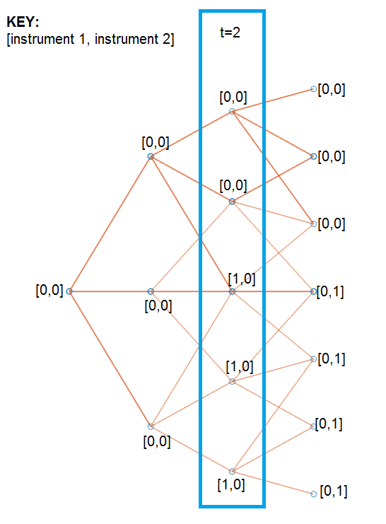
By looking at PriceTree.ExTree, you can determine if the options are exercised. If either of the two instruments has options exercised at t = 2, which is the third level of the tree, the values in ExTree are 1; otherwise, the value is 0.
PriceTree.ExTree{3}ans = 2×5
0 0 1 1 1
0 0 0 0 0
At t = 2, the first instrument has its option exercised at some nodes, while there is no exercise for the second instrument. The following diagram summarizes the exercise indicators on the tree.
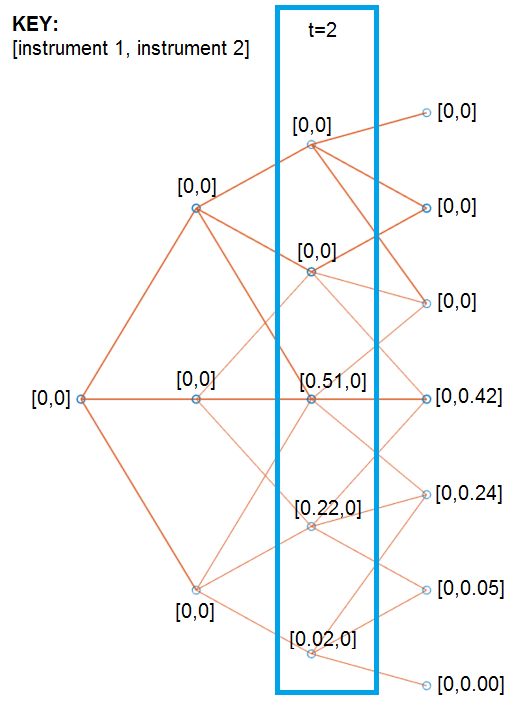
Examine ExProbTree, which contains the exercise probabilities. These values indicate the probability of exercising the option.
PriceTree.ExProbTree{3}ans = 2×5
0 0 0.5087 0.2218 0.0238
0 0 0 0 0
ExProbsByTreeLevel is an aggregated view of ExProbTrees. Examine the exercise probabilities for the two options at each tree observation time.
PriceTree.ExProbsByTreeLevel
ans = 2×5

         0         0    0.7544         0         0
         0         0         0    0.7124         0
The first row corresponds to instrument 1, and the second row corresponds to instrument 2.
You can use treeviewer to examine the tree and PriceTree structures for any of the following tree types: