Unit Root Tests
Test Simulated Data for a Unit Root
This example shows how to test univariate time series models for stationarity. It shows how to simulate data from four types of models: trend stationary, difference stationary, stationary (AR(1)), and a heteroscedastic, random walk model. It also shows that the tests yield expected results.
Simulate four time series.
T = 1e3;       % Sample size
t = (1:T)';    % Time multiple

rng(142857);   % For reproducibility

y1 = randn(T,1) + .2*t; % Trend stationary

Mdl2 = arima(D=1,Constant=0.2,Variance=1);
y2 = simulate(Mdl2,T,Y0=0); % Difference stationary

Mdl3 = arima(AR=0.99,Constant=0.2,Variance=1);
y3 = simulate(Mdl3,T,Y0=0); % AR(1)

Mdl4 = arima(D=1,Constant=0.2,Variance=1);
sigma = (sin(t/200) + 1.5)/2; % Std deviation
e = randn(T,1).*sigma;        % Innovations
y4 = filter(Mdl4,e,Y0=0);   % Heteroscedastic
Plot the first 100 points in each series.
y = [y1 y2 y3 y4];
figure
plot1 = plot(y(1:100,:),LineWidth=2);
plot1(1).LineStyle = ":";
plot1(4).LineStyle = ":";
title("First 100 Periods of Each Series")
legend("Trend Stationary","Difference Stationary","AR(1)", ...
   "Heteroscedastic",Location="northwest")

All of the models appear nonstationary and behave similarly. Therefore, you might find it difficult to distinguish which series comes from which model simply by looking at their initial segments.
Plot the entire data set.
plot2 = plot(y,LineWidth=2);
plot2(1).LineStyle = ":";
plot2(4).LineStyle = ":";
title("Each Entire Series");
legend("Trend Stationary","Difference Stationary","AR(1)", ...
   "Heteroscedastic",Location="NorthWest");

The differences between the series are clearer here:
The trend stationary series has little deviation from its mean trend.
The difference stationary and heteroscedastic series have persistent deviations away from the trend line.
The AR(1) series exhibits long-run stationary behavior; the others grow linearly.
The difference stationary and heteroscedastic series appear similar. However, that the heteroscedastic series has much more local variability near period 300, and much less near period 900. The model variance is maximal when , at time . The model variance is minimal when , at time . Therefore, the visual variability matches the model.
Use the Augmented Dicky-Fuller test on the three growing series (y1, y2, and y4) to assess whether the series have a unit root. Since the series are growing, specify that there is a trend. In this case, the null hypothesis is and the alternative hypothesis is . Set the number of lags to 2 for demonstration purposes.
hY1 = adftest(y1,Model="ts",Lags=2)hY1 = logical
1
hY2 = adftest(y2,Model="ts",Lags=2)hY2 = logical
0
hY4 = adftest(y4,Model="ts",Lags=2)hY4 = logical
0
hY1 = 1indicates that there is sufficient evidence to suggest thaty1is trend stationary. This is the correct decision becausey1is trend stationary by construction.hY2 = 0indicates that there is not enough evidence to suggest thaty2is trend stationary. This is the correct decision sincey2is difference stationary by construction.hY4 = 0indicates that there is not enough evidence to suggest thaty4is trend stationary. This is the correct decision, however, the Dickey-Fuller test is not appropriate for a heteroscedastic series.
Use the Augmented Dickey-Fuller test on the AR(1) series (y3) to assess whether the series has a unit root. Since the series is not growing, specify that the series is autoregressive with a drift term. In this case, the null hypothesis is and the alternative hypothesis is . Set the number of lags to 2 for demonstration purposes.
hY3 = adftest(y3,Model="ard",Lags=2)hY3 = logical
1
hY3 = 1 indicates that there is enough evidence to suggest that y3 is a stationary, autoregressive process with a drift term. This is the correct decision because y3 is an autoregressive process with a drift term by construction.
Use the KPSS test to assess whether the series are unit root nonstationary. Specify that there is a trend in the growing series (y1, y2, and y4). The KPSS test assumes the following model:
where is a stationary process and is an independent and identically distributed process with mean 0 and variance . Whether there is a trend in the model, the null hypothesis is (the series is trend stationary) and the alternative hypothesis is (not trend stationary). Set the number of lags to 2 for demonstration purposes.
hY1 = kpsstest(y1,Lags=2,Trend=true)
hY1 = logical
0
hY2 = kpsstest(y2,Lags=2,Trend=true)
hY2 = logical
1
hY3 = kpsstest(y3,Lags=2)
hY3 = logical
1
hY4 = kpsstest(y4,Lags=2,Trend=true)
hY4 = logical
1
All is tests result in the correct decision.
Use the variance ratio test on al four series to assess whether the series are random walks. The null hypothesis is : is constant, and the alternative hypothesis is : is not constant. Specify that the innovations are independent and identically distributed for all but y1. Test y4 both ways.
hY1 = vratiotest(y1)
hY1 = logical
   1
hY2 = vratiotest(y2,IID=true)
hY2 = logical
   0
hY3 = vratiotest(y3,IID=true)
hY3 = logical
   0
hY4NotIID = vratiotest(y4)
hY4NotIID = logical
   0
hY4IID = vratiotest(y4,IID=true)
hY4IID = logical
   0
All tests result in the correct decisions, except for hY4_2 = 0. This test does not reject the hypothesis that the heteroscedastic process is an IID random walk. This inconsistency might be associated with the random seed.
Alternatively, you can assess stationarity using pptest
Test Time Series Data for Unit Root
This example shows how to test a univariate time series for a unit root. It uses wages data (1900-1970) in the manufacturing sector. The series is in the Nelson-Plosser data set.
Load the Nelson-Plosser data. Extract the nominal wages data.
load Data_NelsonPlosser
wages = DataTable.WN;
Trim the NaN values from the series and the corresponding dates (this step is optional because the test ignores NaN values).
wDates = dates(isfinite(wages));
wages = wages(isfinite(wages));
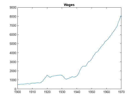
Plot the data to look for trends.
plot(wDates,wages)
title('Wages')
The plot suggests exponential growth.
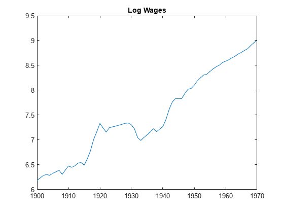
Transform the data using the log function to linearize the series.
logWages = log(wages);
plot(wDates,logWages)
title('Log Wages')
The plot suggests that time series has a linear trend.
Test the null hypothesis that there is no unit root (trend stationary) against the alternative hypothesis that the series is a unit root process with a trend (difference stationary). Set 'Lags',7:2:11, as suggested in Kwiatkowski et al., 1992.
[h1,pValue1] = kpsstest(logWages,'Lags',7:2:11)h1 = 1×3 logical array
0 0 0
pValue1 = 1×3

    0.1000    0.1000    0.1000
kpsstest fails to reject the null hypothesis that the wage series is trend stationary.
Test the null hypothesis that the series is a unit root process (difference stationary) against the alternative hypothesis that the series is trend stationary.
[h2,pValue2] = adftest(logWages,'Model','ts')
h2 = logical
   0
pValue2 =
0.8327
adftest fails to reject the null hypothesis that the wage series is a unit root process.
Because the results of the two tests are inconsistent, it is unclear that the wage series has a unit root. This is a typical result of tests on many macroeconomic series.
kpsstest has a limited set of calculated critical values. When it calculates a test statistic that is outside this range, the test reports the p-value at the appropriate endpoint. So, in this case, pValue reflects the closest tabulated value. When a test statistic lies inside the span of tabulated values, kpsstest linearly interpolates the p-value.
Test Stock Data for Random Walk
This example shows how to assess whether a time series is a random walk. It uses market data for daily returns of stocks and cash (money market) from the period January 1, 2000 to November 7, 2005.
Load the data, which is available only with the Financial Toolbox™ documentation.
load CAPMuniverseThe timetable AssetsTimeTable contains the data. The first column of data in the timetable is the daily return of a technology stock. The last (14th) column is the daily return for cash (the daily money market rate). The returns are the logs of the ratios of values at the end of a day over the values at the beginning of the day.
Because vratiotest takes prices as inputs, as opposed to returns, Convert the data to prices (values) instead of returns.
DTTCS = varfun(@cumsum,AssetsTimeTable,InputVariables=[1 14]);
vnames = AssetsTimeTable.Properties.VariableNames([1 14]);
DTTCS.Properties.VariableNames = vnames;
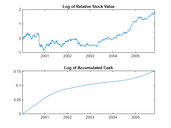
Plot the data to see whether the series appear to be stationary.
figure
tiledlayout(2,1)
nexttile;
plot(DTTCS.Time,DTTCS.AAPL);
title("Log of Relative Stock Value")
nexttile;
plot(DTTCS.Time,DTTCS.CASH)
title("Log of Accumulated Cash")

Cash has small variability, and appears to have long-term trends. The stock series has larger variability, and possibly an upwards trend in the second half of the data.
Test whether the stock series matches a random walk.
[VRTestAAPL1,ratioAAPL1] = vratiotest(DTTCS,DataVariable="AAPL")VRTestAAPL1=1×7 table
0 0.1646 -1.3899 1.9600 0.0500 2 0
ratioAAPL1 =
0.9436
vratiotest does not reject the hypothesis that a random walk is a reasonable model for the stock series.
Test whether an iid random walk is a reasonable model for the stock series.
[VRTestAAPL2,ratioAAPL2] = vratiotest(DTTCS,DataVariable="AAPL",IID=true)VRTestAAPL2=1×7 table
1 0.0304 -2.1642 1.9600 0.0500 2 1
ratioAAPL2 =
0.9436
vratiotest rejects the hypothesis that an iid random walk is a reasonable model for the technology stock series at the 5% level. Thus, vratiotest indicates that the most appropriate model of the technology stock series is a heteroscedastic random walk.
Test whether the cash series matches a random walk.
[VRTestCASH,ratioCASH] = vratiotest(DTTCS,DataVariable="CASH")VRTestCASH=1×7 table
1 4.6093e-145 25.6466 1.9600 0.0500 2 0
ratioCASH =
2.0006
vratiotest rejects the hypothesis that a random walk is a reasonable model for the cash series (pValue = 4.6093e-145). The removal of a trend from the series does not affect the resulting statistics.
References
[1] Kwiatkowski, D., P. C. B. Phillips, P. Schmidt and Y. Shin. “Testing the Null Hypothesis of Stationarity against the Alternative of a Unit Root.” Journal of Econometrics. Vol. 54, 1992, pp. 159–178.
See Also
adftest | kpsstest | pptest | vratiotest