HDL Implementation of LMS Filter

This example uses:

This example shows how to implement a fully serial and transpose delayed least mean square (LMS) adaptive filters. The fully serial LMS filter uses standard LMS adaptive filter algorithm and the transpose delayed LMS filter uses delayed LMS filter algorithm with a transpose filter architecture. You can use the fully serial LMS filter for low data-rate applications, such as audio and speech, and the transpose delayed LMS filter for high throughput applications in wireless communication. For high throughput applications, you can also use the LMS Filter block in DSP HDL Toolbox™. The Simulink® model in this example is optimized for HDL code generation and hardware implementation.

The fully serial and transpose delayed LMS filters minimize the error between a desired signal and an observed signal by adjusting the filter weights using mean square error (MSE) criteria. The example model accepts observed, desired, and step-size signals as input and computes the filtered signal, filter error, and filter weights or coefficients. You can use LMS filters for system identification, inverse system identification, noise cancellation, and prediction.

Fully Serial LMS Filter

The block diagram in this section explains the implementation of a fully serial finite impulse response (FIR) filter architecture along with the LMS algorithm filter weights. In this block diagram, the buffered input samples select the data for each tap serially and multiplies with the corresponding coefficients. This architecture reduces the hardware resource utilization, which generates less number of multipliers with additional logic elements such as multiplexers and registers, when compared to fully parallel implementation of LMS filter. Implementation of this architecture requires a clock rate that is faster than the input sample, which depends on the filter length and the number of delays in the feedback path. For example, for a filter length of 16, the block accepts valid input samples for every 35 clock cycles, which is the filter length plus 19 clock cycles.

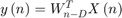
This section explains the LMS equations corresponding to this architecture. The observed signal $x\left(n\right)$ is passed as an input to the filter and buffered for every filter length of samples. This buffered data $X\left(n\right)$ is multiplied serially with the corresponding filter coefficients $W_{n}$ and accumulated in a register to get the filtered output $y\left(n\right)$ at timestep $n$ .

$y\left(n\right) = W_n^T \mathit{X}\left(n\right)$

To get the filter error output at timestep $n$ , subtract the filtered output $y\left(n\right)$ from the desired signal $d\left(n\right)$ .

$e\left(n\right) = d\left(n\right)-y\left(n\right)$

To update the LMS filter weights $W_{n}$ for the next timestep $n+1$ , LMS uses the filter error $e\left(n\right)$ and step size ( $\mu$ ).

${W}_{n+1} = W_{n\;} +\mu e\left(n\right){\mathit{X}}^* \left(n\right)$

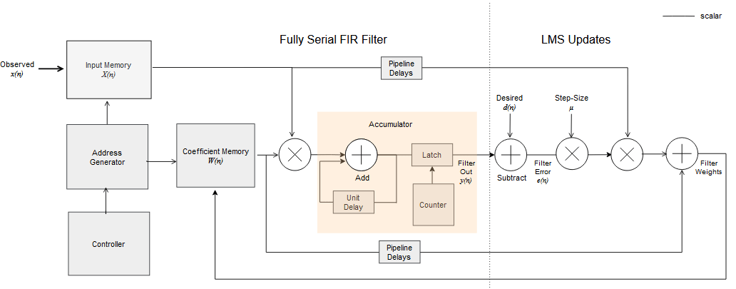
This architecture diagram consists of the fully serial FIR part, $y\left(n\right)$ and the LMS update part, $e\left(n\right)$ and $W_{n+1}$ . The left-side of the diagram shows the fully serial FIR part, and the right-side of the diagram shows the LMS filter weight update part. The input and coefficient memories are used to buffer the observed data and store the filter coefficients.

Model Architecture

Open the example model by entering this command at the MATLAB® command prompt.

modelname = 'HDLFullySerialLMSModel';
open_system(modelname);

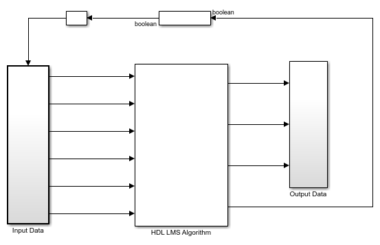
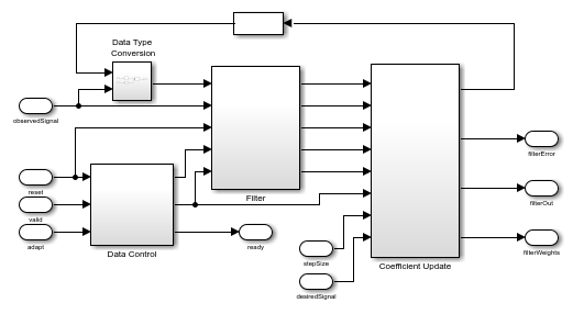
The HDL LMS Algorithm subsystem has Data Control, Filter, and Coefficient Update blocks. The Data Control block generates control signals to control the flow of data. The ready signal indicates when to provide the next valid data. The Filter block implements the serial FIR filter and writes the observed input samples to the RAM. The control logic reads the buffered data serially in such a way that these samples get multiplied with their corresponding filter weights and that the output product is added serially to a register for every filter length of samples to get the filtered output. The Filter block stores the LMS filter weight updates in the RAM and resets the block using a separate reset control logic (when required). The Coefficient Update block implements $e\left(n\right)$ and $W_{n+1}$ of the LMS filter. This example starts with a set of zeros as initial values for the estimates of the filter weights.

open_system([modelname '/HDL LMS Algorithm'],'force')

Transpose Delayed LMS Filter

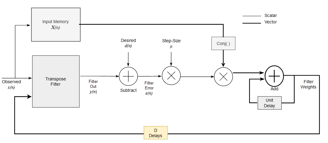
This section explains the equations corresponding to the delayed LMS algorithm. These equations are approximations to the standard LMS algorithm. The transpose delayed LMS filter uses these equations with transpose filter structure to fit the hardware characteristics. The observed signal $x\left(n\right)$ is passed as an input to the filter. The number of delays (D) in the feedback path are independent of filter length because the filter part is implemented using a transposed filter architecture, which improves the throughput by minimizing the pipelined delays in the feedback path of LMS filter.

The filtered output $y\left(n\right)$ at timestep $n$ is given by the equation.

$y\left(n\right) = W_{n-D}^T \mathit{X}\left(n\right)$

To get the filter error output at timestep $n$ , subtract the filtered output $y\left(n\right)$ from the desired signal $d\left(n\right)$ .

$e\left(n\right) = d\left(n\right)-y\left(n\right)$

To update the filter weights $W_{n}$ for the next timestep $n+1$ , LMS filter uses the filter error $e\left(n\right)$ and step size ( $\mu$ ).

${W}_{n+1} = W_{n\;} +\mu e\left(n\right){\mathit{X}}^* \left(n\right)$

This architecture diagram shows the transpose delayed LMS filter.

Model Architecture

Open the example model by entering this command at the MATLAB® command prompt.

modelname = 'HDLDelayedLMSModel';
open_system(modelname);

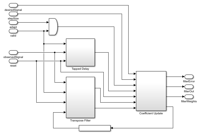
The HDL LMS Algorithm subsystem has Transpose Filter, Tapped Delay, and Coefficient Update blocks. The Transpose filter implements the transpose filter structure and outputs $y\left(n\right)$ . The Tapped delay block buffers the input data $X\left(n\right)$ . The Coefficient Update block implements $e\left(n\right)$ and $W_{n+1}$ of the LMS filter. This example starts with a set of zeros as initial values for the estimates of the filter weights.

open_system([modelname '/HDL LMS Algorithm'],'force')

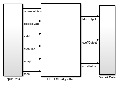
Port and Parameter Descriptions

This section explains the port and parameter descriptions for the HDLFullySerialLMSModel.slx and HDLDelayLMSFilterModel.slx models. The input observedSignal and desiredSignal signals must be scalars and of the same data type. To support HDL code generation, inputs must be scalar fixed-point data types.

Input Ports

observedSignal — Input observed signal $x\left(n\right)$ to the LMS filter, specified as a real- or complex-valued scalar. The block supports double, single, and signed fixed-point data types.
desiredSignal — Input desired signal $d\left(n\right)$ to the LMS filter, specified as a real- or complex-valued scalar. The block supports double, single, and signed fixed-point data types.
stepSize — Input step size $\mu$ to the block, specified as double, single, or unsigned fixed-point data types. This value determines the convergence rate and stability of the filter and must be less than 1/(power of input signal x filter length) for filter stability. For more information, see [ 1 ].
reset — Input reset signal, specified as a Boolean scalar. When reset is true, the block stops the current calculation and clears the internal states.
valid — Input valid signal, specified as a Boolean scalar to validate the input data.
adapt — Input adapt signal, specified as a Boolean scalar. When this signal is 1 (high), the LMS filter updates its filter weights. When this signal is 0 (low), the filter weights remain the same as what they were previously. This signal is sampled only when the valid signal is 1 (high).

Output Ports

fiteredOut — Filtered output $y\left(n\right)$ , returned as a scalar. The LMS filter converges this signal with desired signal $d\left(n\right)$ by adjusting filter weights.
filterError — Filter error $e\left(n\right)$ , returned as a scalar. This value is the difference between filtered output $y\left(n\right)$ and desired signal $d\left(n\right)$ .
filterWeights — Filter weights $W_{n}$ , returned as a scalar for the HDLFullySerialLMSModel.slx model and a vector of the same size as filter length for the HDLDelayLMSFilterModel.slx model.
ready — Ready signal, returned as a Boolean scalar. This port is applicable for the HDLFullySerialLMSModel.slx model. This signal indicates when to provide the next data.

This LMS filter model accepts the filter length as a parameter.

For a fixed-point implementation, internal word length calculations are based on the assumption that the input is a unit power signal. The recommended data type for the inputs and the observed and desired signals is fixdt(1,16,14). The recommended data type for the step size is fixdt(0,18,18).

System Identification of FIR Filter

System identification is a process to find unknown system filter coefficients using an adaptive filter. This section shows how to find unknown system coefficients.

Create a filter object for an unknown system.

filterLength = 16;
filterObj = dsp.FIRFilter;
filterObj.Numerator = fircband(filterLength-1,[0 0.4 0.5 1],[1 1 0 0],[1 0.2],...
    {'w' 'c'});
filterObj %#ok

filterObj = 

  dsp.FIRFilter with properties:

            Structure: 'Direct form'
      NumeratorSource: 'Property'
            Numerator: [-0.0346 0.0069 0.0766 0.0156 ... ] (1x16 double)
    InitialConditions: 0

  Use get to show all properties

Specify a model.

% For the fully serial LMS filter, use 'HDLFullySerialLMSModel', for
% delayed LMS filter use 'HDLDelayedLMSModel'
modelname = 'HDLFullySerialLMSModel';

Pass the unit power signal, observedSignal to the FIR filter. The desiredSignal is the sum of the output of the unknown system (FIR filter) and the additive noise signal noise. The LMS filter adapts its coefficients until its transfer function matches the transfer function of the unknown system.

observedSignal = randn(1500,1);
noise = 0.001*randn(1500,1);
desiredSignal = filterObj(observedSignal) + noise;
stepSize = 0.01;

% Create input and control signals
adaptIn = true(length(observedSignal),1);
resetIn = false(length(observedSignal),1);
validIn = true(length(observedSignal),1);

if strcmpi(modelname,'HDLFullySerialLMSModel')
    simtime = length(observedSignal)*(filterLength+19) + 10;
else
    simtime = length(observedSignal) + 100;
end
out = sim(modelname);

% Capture valid data outputs
actFilterOut = out.filterOut;
actCoeffOut = out.coeffOut;
actErrorOut = out.errorOut;

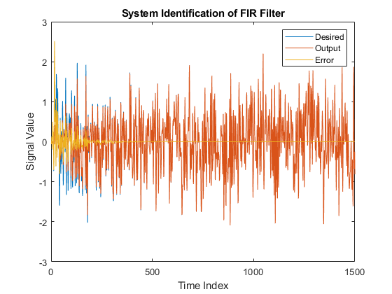
Plot the outputs.

figure;
plot(1:1:length(observedSignal),double([desiredSignal,actFilterOut,actErrorOut]))
title('System Identification of FIR Filter')
legend('Desired','Output','Error')
xlabel('Time Index')
ylabel('Signal Value')

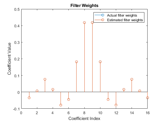
Because the output weights for the HDLFullySerialLMSModel.slx model are serial, you must convert the weights to a vector to represent the coefficients of the LMS filter, which is adapted to resemble the unknown system (FIR filter). To confirm the convergence, compare the numerator of the FIR filter with the estimated weights of the LMS filter.

figure;
% Compare actual filter weights with estimated filter weights
if strcmpi(modelname,'HDLFullySerialLMSModel')
    val = (filterLength)*(length(observedSignal)-1);
    stem([(filterObj.Numerator).' double(actCoeffOut((val+1):(val+filterLength)))]);
else
    val = (length(observedSignal)-1);
    stem([(filterObj.Numerator).' double(actCoeffOut((val+1),:)).']);
end
xlabel('Coefficient Index')
ylabel('Coefficient Value')
title('Filter Weights')
legend('Actual filter weights','Estimated filter weights', ...
    'Location','NorthEast')

Verification and Results

For verification, compare the outputs from this example with the outputs from the dsp.LMSFilter function.

lms = dsp.LMSFilter(filterLength,'StepSize',stepSize);
[y,e,w] = lms(observedSignal,desiredSignal);

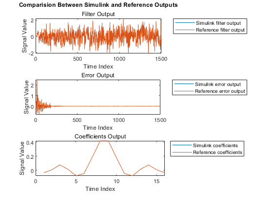
Plot the Simulink and reference outputs and verify the difference between them.

figure;
% Compare Simulink and reference filtered out
subplot(3,1,1)
plot(1:length(observedSignal),[actFilterOut,y])
title('Comparision Between Simulink and Reference Outputs')
subtitle('Filter Output')
legend('Simulink filter output','Reference filter output','Location','bestoutside')
xlabel('Time Index')
ylabel('Signal Value')

% Compare Simulink and reference filter error out
subplot(3,1,2);
plot(1:length(observedSignal),[actErrorOut,e])
subtitle('Error Output')
legend('Simulink error output','Reference error output','Location','bestoutside')
xlabel('Time Index')
ylabel('Signal Value')

% Compare Simulink and reference filtered coefficients
subplot(3,1,3);
if strcmpi(modelname,'HDLFullySerialLMSModel')
    plot(1:filterLength,[double(actCoeffOut((val+1):(val+filterLength))),w])
else
    plot(1:filterLength,[double(actCoeffOut((val+1),:)).',w])
end
subtitle('Coefficients Output')
legend('Simulink coefficients','Reference coefficients','Location','bestoutside')
xlabel('Time Index')
ylabel('Signal Value')

Noise Cancellation Using LMS Filter

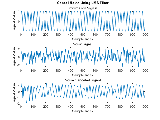
Run the HDLLMSNoiseRemoval.m script to remove noise from the information signal. The information signal is a pure sine wave corrupted with additive noise, which is considered as a desired signal. The observed signal is correlated with noise data and fed to the LMS filter. When the filter converges, it provides the noise-canceled information signal from the filterError port. This plot shows the information signal, noisy signal, and the output noise corrected signal from the fully serial LMS filter in the HDLFullySerialLMSModel.slx model. You can generate similar plot for the transpose delayed LMS filter by specifying the model HDLDelayedLMSModel.slx in the HDLLMSNoiseRemoval.m script.

>> HDLLMSNoiseRemoval

HDLLMSNoiseRemoval

Mean Square Performance

Run the HDLLMSConvergencePlot.m script to plot the mean square error (MSE) performance of the LMS algorithm. The MSE measures the average squares of the errors between the desired signal and the primary input signal to the adaptive filter. This plot is the convergence plot for the fully serial LMS filter in the HDLFullySerialLMSModel.slx model and the transpose delayed LMS filter in the HDLDelayedLMSModel.slx model. The convergence plot of the transpose delayed LMS filter for the small step sizes closely matches with the fully serial LMS filter.

>> HDLLMSConvergencePlot

HDLLMSConvergencePlot

Throughput

The throughput for the fully serial LMS filter in the HDLFullySerialLMSModel.slx model is calculated as (fMax / (FL + t)). The throughput for transpose delayed LMS filter in the HDLDelayedLMSModel.slx model is equivalent to fMax , which is independent of the filter length. In this calculation: fMax is the maximum operating frequency, FL is the filter length, and t is the number of pipeline delays required in feedback path of fully serial LMS implementation. t is 19 in this implementation.

HDL Code Generation and Implementation Results

To generate HDL code for this example, you must have HDL Coder™ product. To generate HDL code and HDL test bench, use the makehdl and makehdltb commands. The block is synthesized on a Xilinx® Zynq®-7000 ZC706 evaluation board.

For the fully serial LMS filter in the HDLFullySerialLMSModel.slx model, this example achieves a clock frequency of 470 MHz. For the transpose delayed LMS filter in the HDLDelayedLMSModel.slx model, this example achieves a clock frequency of 450 MHz. These tables show the post place and route resource utilization results for the real-valued input word length of 16 and step-size word length of 18 for a filter length of 16 for both models. The resource utilization and synthesis frequency vary with the filter length and input word lengths.

Display the resource utilization for the fully serial LMS filter in the HDLFullySerialLMSModel.slx model.

F = table( ...
    categorical({'Slice Registers'; 'Slice LUT';'DSP'}), ...
    categorical({'551'; '412'; '3'}), ...
    categorical({'437200'; '218600'; '900'}), ...
    categorical({'0.13'; '0.19'; '0.33'}), ...
    'VariableNames',{'Resources','Utilized','Available','Utilization (%)'});
disp(F)

       Resources       Utilized    Available    Utilization (%)
    _______________    ________    _________    _______________

    Slice Registers      551        437200           0.13      
    Slice LUT            412        218600           0.19      
    DSP                  3          900              0.33

Display the resource utilization for the transpose delayed LMS filter in HDLDelayedLMSModel.slx model.

F = table( ...
    categorical({'Slice Registers'; 'Slice LUT';'DSP'}), ...
    categorical({'3395'; '2914'; '33'}), ...
    categorical({'437200'; '218600'; '900'}), ...
    categorical({'0.78'; '1.33'; '3.67'}), ...
    'VariableNames',{'Resources','Utilized','Available','Utilization (%)'});
disp(F)

       Resources       Utilized    Available    Utilization (%)
    _______________    ________    _________    _______________

    Slice Registers      3395       437200           0.78      
    Slice LUT            2914       218600           1.33      
    DSP                  33         900              3.67

References

[1] Hayes,M.H. Statistical Digital Signal Processing and Modeling. New York: John Wiley & Sons, 1996.