Create an FIR Filter Using Integer Coefficients
This section provides an example of how you can create a filter with integer coefficients. In this example, a raised-cosine filter with floating-point coefficients is created, and the filter coefficients are then converted to integers.
Define the Filter Coefficients
To illustrate the concepts of using integers with fixed-point filters, this example will use a raised-cosine filter:
b = rcosdesign(.25, 12.5, 8, 'sqrt');
b are normalized so that the passband
gain is equal to 1, and are all smaller than 1. In order to make them
integers, they will need to be scaled. If you wanted to scale them
to use 18 bits for each coefficient, the range of possible values
for the coefficients becomes:
Because the largest
coefficient of b is positive, it will need to be
scaled as close as possible to 131071 (without overflowing) in order
to minimize quantization error. You can determine the exponent of
the scale factor by executing:
B = 18; % Number of bits
L = floor(log2((2^(B-1)-1)/max(b)));  % Round towards zero to avoid overflow
bsc = b*2^L;
Alternatively, you can use the fixed-point numbers autoscaling tool as follows:
bq = fi(b, true, B);  % signed = true, B = 18 bits
L = bq.FractionLength;
It is a coincidence that B and L are
both 18 in this case, because of the value of the largest coefficient
of b. If, for example, the maximum value of b were
0.124, L would be 20 while B (the
number of bits) would remain 18.
Build the FIR Filter
First create the filter using the direct form, tapped delay line structure:
h = dfilt.dffir(bsc);
In order to set the required parameters, the arithmetic must be set to fixed-point:
h.Arithmetic = 'fixed';
h.CoeffWordLength = 18;
You can check that the coefficients of h are
all integers:
all(h.Numerator == round(h.Numerator))

ans =

	1
Now you can examine the magnitude response of the filter using fvtool:
fvtool(h, 'Color', 'white')
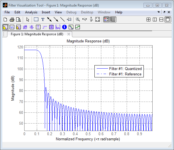
This shows a large gain of 117 dB in the passband, which is due to the large values of the coefficients— this will cause the output of the filter to be much larger than the input. A method of addressing this will be discussed in the following sections.
Set the Filter Parameters to Work with Integers
You will need to set the input parameters of your filter to appropriate values for working with integers. For example, if the input to the filter is from a A/D converter with 12 bit resolution, you should set the input as follows:
h.InputWordLength = 12;
h.InputFracLength = 0;
The info method returns a summary of the
filter settings.
info(h)
Discrete-Time FIR Filter (real)
-------------------------------
Filter Structure  : Direct-Form FIR
Filter Length     : 101
Stable            : Yes
Linear Phase      : Yes (Type 1)
Arithmetic        : fixed
Numerator         : s18,0 -> [-131072 131072)
Input             : s12,0 -> [-2048 2048)
Filter Internals  : Full Precision
  Output          : s31,0 -> [-1073741824 1073741824)  (auto determined)
  Product         : s29,0 -> [-268435456 268435456)  (auto determined)
  Accumulator     : s31,0 -> [-1073741824 1073741824)  (auto determined)
  Round Mode      : No rounding
  Overflow Mode   : No overflow
In this case, all the fractional lengths are now set to zero,
meaning that the filter h is set up to handle integers.
Create a Test Signal for the Filter
You can generate an input signal for the filter by quantizing to 12 bits using the autoscaling feature, or you can follow the same procedure that was used for the coefficients, discussed previously. In this example, create a signal with two sinusoids:
n = 0:999;
f1 = 0.1*pi;  % Normalized frequency of first sinusoid
f2 = 0.8*pi;  % Normalized frequency of second sinusoid
x = 0.9*sin(0.1*pi*n) + 0.9*sin(0.8*pi*n);
xq = fi(x, true, 12);  % signed = true, B = 12
xsc = fi(xq.int, true, 12, 0);
Filter the Test Signal
To filter the input signal generated above, enter the following:
ysc = filter(h, xsc);
Here ysc is a full precision output, meaning
that no bits have been discarded in the computation. This makes ysc the
best possible output you can achieve given the 12–bit input
and the 18–bit coefficients. This can be verified by filtering
using double-precision floating-point and comparing the results of
the two filtering operations:
hd = double(h);
xd = double(xsc);
yd = filter(hd, xd);
norm(yd-double(ysc))

ans =

     0
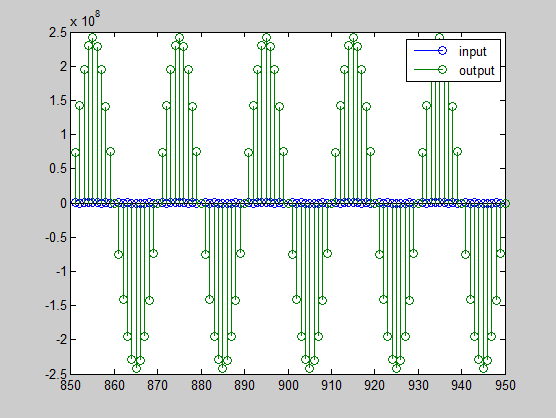
Now you can examine the output compared to the input. This example is plotting only the last few samples to minimize the effect of transients:
idx = 800:950;
xscext = double(xsc(idx)');
gd = grpdelay(h, [f1 f2]);
yidx = idx + gd(1);
yscext = double(ysc(yidx)');
stem(n(idx)', [xscext, yscext]);
axis([800 950 -2.5e8 2.5e8]);
legend('input', 'output');
set(gcf, 'color', 'white');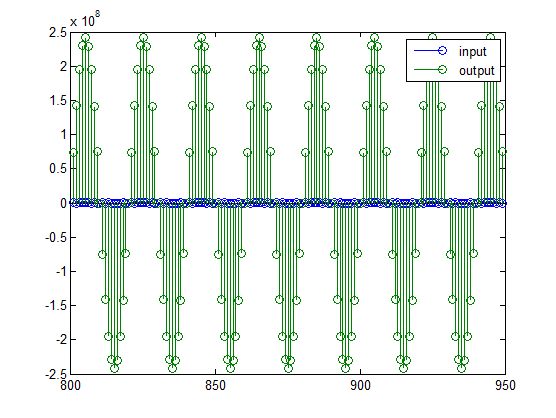
It is difficult to compare the two signals in this figure because of the large difference in scales. This is due to the large gain of the filter, so you will need to compensate for the filter gain:
stem(n(idx)', [2^18*xscext, yscext]);
axis([800 950 -5e8 5e8]);
legend('scaled input', 'output');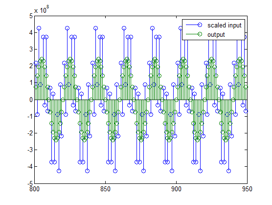
You can see how the signals compare much more easily once the scaling has been done, as seen in the above figure.
Truncate the Output WordLength
If you examine the output wordlength,
ysc.WordLength

ans =

    31
you will notice that the number of bits in the output is considerably greater than in the input. Because such growth in the number of bits representing the data may not be desirable, you may need to truncate the wordlength of the output. The best way to do this is to discard the least significant bits, in order to minimize error. However, if you know there are unused high order bits, you should discard those bits as well.
To determine if there are unused most significant bits (MSBs),
you can look at where the growth in WordLength arises in the computation.
In this case, the bit growth occurs to accommodate the results of
adding products of the input (12 bits) and the coefficients (18 bits).
Each of these products is 29 bits long (you can verify this using info(h)).
The bit growth due to the accumulation of the product depends on the
filter length and the coefficient values- however, this is a worst-case
determination in the sense that no assumption on the input signal
is made besides, and as a result there may be unused MSBs. You will
have to be careful though, as MSBs that are deemed unused incorrectly
will cause overflows.
Suppose you want to keep 16 bits for the output. In this case, there is no bit-growth due to the additions, so the output bit setting will be 16 for the wordlength and –14 for the fraction length.
Since the filtering has already been done, you can discard some
bits from ysc:
yout = fi(ysc, true, 16, -14);
Alternatively, you can set the filter output bit lengths directly (this is useful if you plan on filtering many signals):
specifyall(h);
h.OutputWordLength = 16;
h.OutputFracLength = -14;
yout2 = filter(h, xsc);
You can verify that the results are the same either way:
norm(double(yout) - double(yout2))

ans =

     0
However, if you compare this to the full precision output, you will notice that there is rounding error due to the discarded bits:
norm(double(yout)-double(ysc))

ans =

    1.446323386867543e+005
In this case the differences are hard to spot when plotting the data, as seen below:
stem(n(yidx), [double(yout(yidx)'), double(ysc(yidx)')]);
axis([850 950 -2.5e8 2.5e8]);
legend('Scaled Input', 'Output');
set(gcf, 'color', 'white');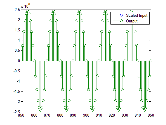
Scale the Output
Because the filter in this example has such a large gain, the output is at a different scale than the input. This scaling is purely theoretical however, and you can scale the data however you like. In this case, you have 16 bits for the output, but you can attach whatever scaling you choose. It would be natural to reinterpret the output to have a weight of 2^0 (or L = 0) for the LSB. This is equivalent to scaling the output signal down by a factor of 2^(-14). However, there is no computation or rounding error involved. You can do this by executing the following:
yri = fi(yout.int, true, 16, 0);
stem(n(idx)', [xscext, double(yri(yidx)')]);
axis([800 950 -1.5e4 1.5e4]);
legend('input', 'rescaled output');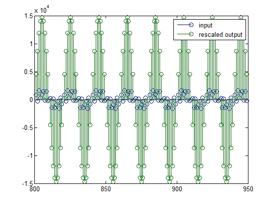
This plot shows that the output is still larger than the input. If you had done the filtering in double-precision floating-point, this would not be the case— because here more bits are being used for the output than for the input, so the MSBs are weighted differently. You can see this another way by looking at the magnitude response of the scaled filter:
[H,w] = freqz(h);
plot(w/pi, 20*log10(2^(-14)*abs(H)));
This plot shows that the passband gain is still above 0 dB.
To put the input and output on the same scale, the MSBs must be weighted equally. The input MSB has a weight of 2^11, whereas the scaled output MSB has a weight of 2^(29–14) = 2^15. You need to give the output MSB a weight of 2^11 as follows:
yf = fi(zeros(size(yri)), true, 16, 4);
yf.bin = yri.bin;
stem(n(idx)', [xscext, double(yf(yidx)')]);
legend('input', 'rescaled output');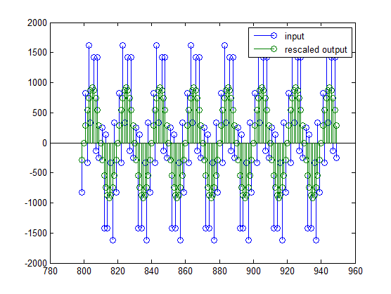
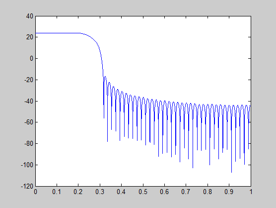
This operation is equivalent to scaling the filter gain down by 2^(-18).
[H,w] = freqz(h);
plot(w/pi, 20*log10(2^(-18)*abs(H)));
The above plot shows a 0 dB gain in the passband, as desired.
With this final version of the output, yf is
no longer an integer. However this is only due to the interpretation-
the integers represented by the bits in yf are
identical to the ones represented by the bits in yri.
You can verify this by comparing them:
max(abs(yf.int - yri.int))

ans =

      0
Configure Filter Parameters to Work with Integers Using the set2int Method
Set the Filter Parameters to Work with Integers
The set2int method provides a convenient
way of setting filter parameters to work with integers. The method
works by scaling the coefficients to integer numbers, and setting
the coefficients and input fraction length to zero. This makes it
possible for you to use floating-point coefficients directly.
h = dfilt.dffir(b);
h.Arithmetic = 'fixed';
The coefficients are represented with 18 bits and the input signal is represented with 12 bits:
g = set2int(h, 18, 12);
g_dB = 20*log10(g)

g_dB =

    1.083707984390332e+002
The set2int method returns the gain of the
filter by scaling the coefficients to integers, so the gain is always
a power of 2. You can verify that the gain we get here is consistent
with the gain of the filter previously. Now you can also check that
the filter h is set up properly to work with integers:
info(h)
Discrete-Time FIR Filter (real)
-------------------------------
Filter Structure  : Direct-Form FIR
Filter Length     : 101
Stable            : Yes
Linear Phase      : Yes (Type 1)
Arithmetic        : fixed
Numerator         : s18,0 -> [-131072 131072)
Input             : s12,0 -> [-2048 2048)
Filter Internals  : Full Precision
  Output     : s31,0 -> [-1073741824 1073741824) (auto determined)
  Product    : s29,0 -> [-268435456 268435456) (auto determined)
  Accumulator: s31,0 -> [-1073741824 1073741824) (auto determined)
  Round Mode      : No rounding
  Overflow Mode   : No overflow
Here you can see that all fractional lengths are now set to zero, so this filter is set up properly for working with integers.
Reinterpret the Output
You can compare the output to the double-precision floating-point
reference output, and verify that the computation done by the filter h is
done in full precision.
yint = filter(h, xsc);
norm(yd - double(yint))

ans =

     0
You can then truncate the output to only 16 bits:
yout = fi(yint, true, 16);
stem(n(yidx), [xscext, double(yout(yidx)')]);
axis([850 950 -2.5e8 2.5e8]);
legend('input', 'output');
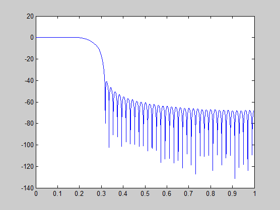
Once again, the plot shows that the input and output are at different scales. In order to scale the output so that the signals can be compared more easily in a plot, you will need to weigh the MSBs appropriately. You can compute the new fraction length using the gain of the filter when the coefficients were integer numbers:
WL = yout.WordLength;
FL = yout.FractionLength + log2(g);
yf2 = fi(zeros(size(yout)), true, WL, FL);
yf2.bin = yout.bin;

stem(n(idx)', [xscext, double(yf2(yidx)')]);
axis([800 950 -2e3 2e3]);
legend('input', 'rescaled output');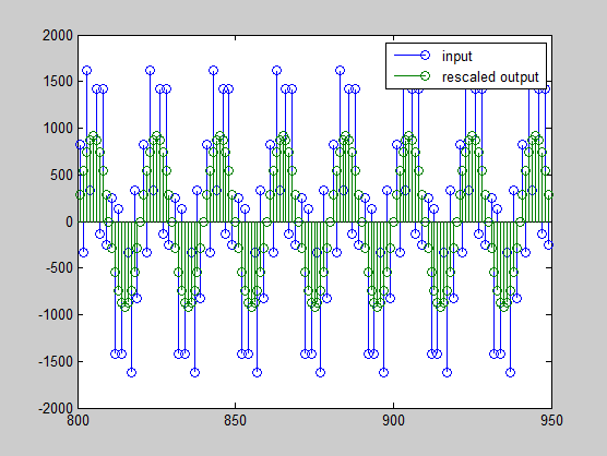
This final plot shows the filtered data re-scaled to match the input scale.