Residual Analysis

Plotting and Analysing Residuals

The residuals from a fitted model are defined as the differences between the response data and the fit to the response data at each predictor value.

residual = data – fit

You can display the residuals in the Curve Fitter app by clicking Residuals Plot in the Visualization section of the Curve Fitter tab.

Mathematically, the residual for a specific predictor value is the difference between the response value y and the predicted response value ŷ.

r = y – ŷ

Assuming the model you fit to the data is correct, the residuals approximate the random errors. Therefore, if the residuals appear to behave randomly, it suggests that the model fits the data well. However, if the residuals display a systematic pattern, it is a clear sign that the model fits the data poorly. Always bear in mind that many results of model fitting, such as confidence bounds, will be invalid should the model be grossly inappropriate for the data.

A graphical display of the residuals for a first-degree polynomial fit is shown below. The top plot shows that the residuals are calculated as the vertical distance from the data point to the fitted curve. The bottom plot displays the residuals relative to the fit, which is the zero line.

The residuals appear randomly scattered around zero indicating that the model describes the data well.

A graphical display of the residuals for a second-degree polynomial fit is shown below. The model includes only the quadratic term, and does not include a linear or constant term.

The residuals are systematically positive for much of the data range indicating that this model is a poor fit for the data.

Example: Residual Analysis

This example fits several polynomial models to generated data and evaluates how well those models fit the data and how precisely they can predict. The data is generated from a cubic curve, and there is a large gap in the range of the x variable where no data exist.

x = [1:0.1:3 9:0.1:10]';
c = [2.5 -0.5 1.3 -0.1]; 
y = c(1) + c(2)*x + c(3)*x.^2 + c(4)*x.^3 + (rand(size(x))-0.5);

Fit the data in the Curve Fitter app using a cubic polynomial and a fifth-degree polynomial. The data, fits, and residuals are shown below. You can display residuals in the Curve Fitter app by clicking Residuals Plot in the Visualization section of the Curve Fitter tab.

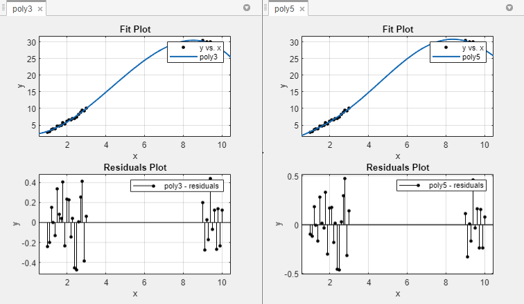
Both models appear to fit the data well, and the residuals appear to be randomly distributed around zero. Therefore, a graphical evaluation of the fits does not reveal any obvious differences between the two equations.

Look at the numerical fit results in the Results pane and compare the confidence bounds for the coefficients.

The results show that the cubic fit coefficients are accurately known (bounds are small), while the quintic fit coefficients are not accurately known. As expected, the fit results for poly3 are reasonable because the generated data follows a cubic curve. The 95% confidence bounds on the fitted coefficients indicate that they are acceptably precise. However, the 95% confidence bounds for poly5 indicate that the fitted coefficients are not known precisely.

The goodness-of-fit statistics are shown in the Table Of Fits pane. By default, the adjusted R-square and RMSE statistics are displayed in the table. The statistics do not reveal a substantial difference between the two equations. To choose statistics to display or hide, right-click the column headers.

The 95% nonsimultaneous prediction bounds for new observations are shown below. To display prediction bounds in the Curve Fitter app, select 95% from the Prediction Bounds list in the Visualization section of the Curve Fitter tab.

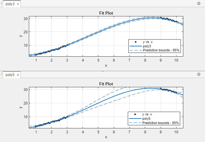
The prediction bounds for poly3 indicate that new observations can be predicted with a small uncertainty throughout the entire data range. This is not the case for poly5. It has wider prediction bounds in the area where no data exist, apparently because the data does not contain enough information to estimate the higher degree polynomial terms accurately. In other words, a fifth-degree polynomial overfits the data.

The 95% prediction bounds for the fitted function using poly5 are shown below. As you can see, the uncertainty in predicting the function is large in the center of the data. Therefore, you would conclude that more data must be collected before you can make precise predictions using a fifth-degree polynomial.

In conclusion, you should examine all available goodness-of-fit measures before deciding on the fit that is best for your purposes. A graphical examination of the fit and residuals should always be your initial approach. However, some fit characteristics are revealed only through numerical fit results, statistics, and prediction bounds.