Field Analysis of Monopole Antenna

This example shows how to conduct the field analysis of monopole antenna using pattern function.

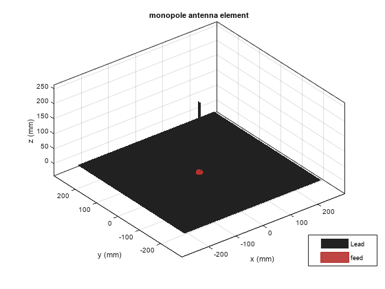
Construct and Visualize Antenna

Use the design function to create a monopole antenna at 300 MHz. Use lead as the conductor material for the antenna.

f=300e6;
ant=design(monopole(Conductor=metal('Lead')),f);
figure;
show(ant)

Compute Directivity, Gain, and Realized Gain

Use the Type name-value pair in the pattern function to visualize the directivity, gain, and realized gain of the monopole antenna.

• directivity

figure;
pattern(ant,f,Type='directivity')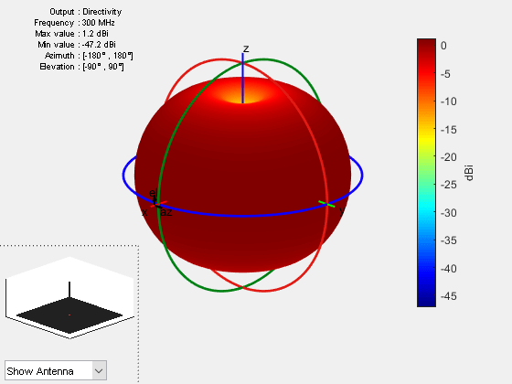

• gain

figure;
pattern(ant,f,Type='gain')

• realized gain

figure;
pattern(ant,f,Type='realizedgain')

Use the max function in dB scale to compute the maximum value of the corresponding 3D patterns.

Dmax=max(max(pattern(ant,f,Type='directivity')))

Dmax = 
1.2046

Gmax=max(max(pattern(ant,f,Type='gain')))

Gmax = 
-1.4579

RGmax=max(max(pattern(ant,f,Type='realizedgain')));

Calculate the radiation efficiency using the efficiency function and the port reflection loss using the S-parameters function.

DiffGminusD=Gmax-Dmax

DiffGminusD = 
-2.6625

EfficiencyValue=10*log10(efficiency(ant,f))

EfficiencyValue = 
-2.6625

s=sparameters(ant,f);
s11=s.Parameters;
ReflectionLoss=10*log10(1-(abs(s11))^2)

ReflectionLoss = 
-0.0495

DiffRGminusG=RGmax-Gmax

DiffRGminusG = 
-0.0495

You see that the efficiency value is the difference between the maximum gain and maximum directivity. The difference between the realized gain and gain values is equal to the port efficiency.

To visualize the maximum amplitude normalize pattern, set Normalize name-value pair in the pattern function to true.

figure;
pattern(ant,f,Type='directivity',Normalize=true)

You can see in the figure that with Normalize name-value pair set to true the maximum gain value is 0 dB.

Calculate Electric Field Magnitude and Norm

To visualize the electric field magnitude set the Type name-value pair to efield.

figure;
pattern(ant,f,Type='efield')

To visualize the norm of the electric field in absolute scale set the Type name-value pair to power.

figure;
pattern(ant,f,Type='power')

To visualize the norm of the electric field in dB scale set the Type name-value pair to powerdB.

figure;
pattern(ant,f,Type='powerdb')

The unit of power when Type is set to power is Watt and when set to powerdB, it is dBW. The Type set to power provides the norm of the electric field at each observation location over the far field radiation sphere. The radiated power of the antenna or the array is different from the power obtained when the Type is set to power. The second one is${\left|\underset{\mathit{s}}{\overset{\mathrm{abs}}{\mathit{E}\left(\mathit{R},\theta ,\varphi \right)}}\right|}^2$ in volt per meter squared. However, the radiated power of the antenna or array is

$$\underset{\mathrm{rad}}{\mathit{P}}={\int }_{\theta =0}^{\Pi }{\int }_{\varphi =0}^{2\Pi }\mathit{U}\left(\theta ,\varphi \right)\sin \theta \mathit{d}\theta \mathit{d}\varphi ={\int }_{\theta =0}^{\Pi }{\int }_{\varphi =0}^{2\Pi }\frac{{\mathit{R}}^2}{2{\eta }_0^{}}{\left|{\mathit{E}}_{\mathit{s}}^{\mathrm{abs}}\left(\mathit{R},\theta ,\varphi \right)\right|}^2\sin \theta \mathit{d}\theta \mathit{d}\varphi$$

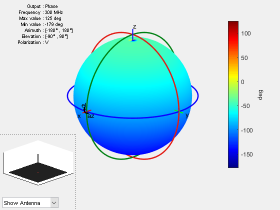
Compute Electric Field Phase

The electric field computed at each observation point over the radiation sphere is a 3-by-1 complex vector. In Cartesian coordinates this vector is written as

$${\mathit{E}}_{\mathit{s}}^{}=\left[\begin{array}{c}{\mathit{E}}_{\mathit{x}}^{}\\ {\mathit{E}}_{\mathit{y}}^{}\\ {\mathit{E}}_{\mathit{z}}^{}\end{array}\right]$$

In the far-field region, the radial component of the electric field becomes zero. The equivalent component of the electric field in the spherical coordinate is:

$${\mathit{E}}_{\theta }^{}={\mathit{E}}_{\mathit{x}}^{}*\cos \theta *\cos \varphi +{\mathit{E}}_{\mathit{y}}^{}*\cos \theta *\cos \varphi -{\mathit{E}}_{\mathit{z}}^{}*\sin \theta$$

$${\mathit{E}}_{\varphi }^{}=-{\mathit{E}}_{\mathit{x}}^{}*\sin \varphi +{\mathit{E}}_{\mathit{y}}^{}*\cos \varphi$$

For a spherical coordinate system, you can use azimuth and elevation angles instead of theta and phi.

azimuth = $\theta$

elevation = $90-\theta$

To compute the phase, you need to specify the polarization in the pattern.

Compute the phase of the electric field with vertical polarization.

figure;
pattern(ant,f,Type='phase',Polarization='V')

Embedded Pattern in Antenna Array

For antenna arrays, the embedded pattern is the pattern obtained by exciting one antenna port and terming the other antenna ports to a certain termination impedance. To plot the embedded element pattern of an array, set the element index ElementNumber property in pattern function. While computing the embedded pattern, you can terminate the antenna’s excitation port to a customized impedance using the Termination property in pattern function. The termination impedance will influence the port efficiency ($\mathrm{PE}=1-{\left|{\mathit{S}}_{11}^{}\right|}^2$ for a single port antenna) and the realized gain depends on the termination impedance value. To have a comparative overview, consider a default four-element rectangular array with two different termination impedance values.

l=rectangularArray;
figure;
show(l)

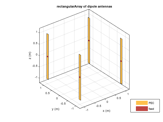
pat1=pattern(l,70e6,0,-90:5:90,ElementNumber=1, Termination=50,...
    Type='realizedgain',CoordinateSystem='rectangular');
pat2= pattern(l,70e6,0,-90:5:90,ElementNumber=1,Termination=200,...
    Type='realizedgain',CoordinateSystem='rectangular');
figure;
plot(-90:5:90,pat1,'r')
hold on
plot(-90:5:90,pat2,'--b')
xlabel('Angle (in degree)')
ylabel('Realized Gain (in dB)')
legend('Termination Imp=50 Ohm','Termination Imp=200 Ohm')