Comparison of Antenna Array Transmit and Receive Manifold
This example calculates and compares the transmit and receive manifolds for a basic half-wavelength dipole antenna array. The array manifold is a fundamental property of antenna arrays, both in transmit and receive configurations. The transmit and receive manifolds are theoretically the same due to the reciprocity theorem. This example validates this equality thus providing an important verification of the calculations performed by the Antenna Toolbox™.
Analysis Setup
Define the variables necessary for calculating the transmit and receive manifolds of an antenna. The frequency for the analysis is 300 MHz which results in a free-space wavelength of approximately 1. Define the sweep angles for azimuth and elevation. These variables are then used to calculate the positions in the far-field of the antenna at which the electric and magnetic fields are computed.
fc = 3e8;
lambda = physconst("lightspeed")/fc;
R = 100*lambda;
M = 4;
ZL = [];
phi = 5:5:175;
psi = 0:5:80;
nphi = length(phi);
npsi = length(psi);
np = nphi*npsi;
PHI = kron(ones(1,npsi),pi/180*phi);
PSI = kron(pi/180*psi,ones(1,nphi));
Create Cartesian Co-ordinates for Observation and Unit Vectors
The azimuth and elevation angle variables are used to calculate the points on a sphere with radius of and the unit vectors.
antennapos = [[-(M-1)/2:(M-1)/2]*lambda/2;zeros(2,M)]';
x = R*cos(PSI).*cos(PHI);
y = R*cos(PSI).*sin(PHI);
z = R*sin(PSI);

Points = [x;y;z];

h = [-sin(PHI);cos(PHI);zeros(size(PHI))];
v = [-cos(PHI).*sin(PSI);-sin(PHI).*sin(PSI);cos(PSI)];
u = [cos(PHI).*cos(PSI);sin(PHI).*cos(PSI);sin(PSI)];
Create Antenna Array
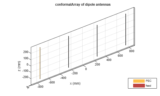
Create a half-wavelength dipole antenna, positioned vertically along the z-axis. Use this element to build a conformal array of dipoles arranged in a linear configuration with half-wavelength spacing between elements.
d = dipole(Length=lambda/2,Width=lambda/200);
elem = [d,d,d,d];
dA = conformalArray(Element=elem,ElementPosition=antennapos);
figure
show(dA)
Compute Array Transmit Manifold
Use EHfields to calculate the electric and magnetic field vectors in the transmit mode for the array. The field calculation at 300 MHz is done at the observation points specified on the far-field sphere and considering the vertical polarization contribution explicitly since the dipole orientation is vertical. The analysis is conducted such that the element under excitation has a load in series with the voltage source, and all other elements, which are not under excitation, do not have any internal impedance.
nomLoad = lumpedElement(Impedance=ZL);
actLoad = lumpedElement(Impedance=50);
for i=[1,1:M]
    % setup loads
    for m=1:M
        dA.Element(m).Load = nomLoad;
    end
    dA.Element(i).Load = actLoad;
    % setup active element
    ampTaper = zeros(1,M);
    ampTaper(i) = 1;
    dA.AmplitudeTaper = ampTaper;
    [E,H] = EHfields(dA,fc,Points);
    Etx(i,:) = sum(E.*v);
end
Compute Array Receive Manifold
To calculate the receive manifold, consider a plane wave incident upon the array with the same electric field polarization but opposite in direction to the transmit mode. Use the planeWaveExcitation object and the feedCurrent function to compute the current passing through the feeds in response to the impinging plane wave.
nomLoad = lumpedElement(Impedance=ZL);
for m=1:M
    dA.Element(m).Load = nomLoad;
end

for n = 1:np
    dirVec = -u(:,n);
    polVec =  v(:,n);
    p = planeWaveExcitation(Element=dA,Direction=dirVec,Polarization=polVec);
    Erx(:,n) = feedCurrent(p,fc).';
end
Compute Normalized Error Between Manifolds
Calculate the normalized error between the transmit and receive manifolds for each element in the array. Reshape the error to plot as a function of the azimuth and elevation angles respectively
for i=1:M
    a(i) = Erx(i,:)/Etx(i,:);
    err(i,:) = abs(Erx(i,:)-a(i)*Etx(i,:));
    mse = sqrt(mean(abs(a(i)*Etx(i,:)).*abs(Erx(i,:))));
    err(i,:) = err(i,:)/mse;
    Etx(i,:) = a(i)*Etx(i,:);
end

ETX = reshape(Etx,M,nphi,npsi);
ERX = reshape(Erx,M,nphi,npsi);
for i = 1:M
    ETXmag(i,:,:) = abs(squeeze(ETX(i,:,:)))';
    ETXphase(i,:,:) = 180/pi*angle(squeeze(ETX(i,:,:)))';
    ERXmag(i,:,:) = abs(squeeze(ERX(i,:,:)))';
    ERXphase(i,:,:) = 180/pi*angle(squeeze(ERX(i,:,:)))';
end
ERR = 20*log10(reshape(mean(err),nphi,npsi));
Plot Transmit and Receive Manifold, and Error Pattern
The transmit and receive manifolds show a great degree of similarity in the magnitude and phase plots. This is confirmed by the error plot with a maximum error of approximately -40 dB over the span of azimuth and elevation angles.
for i=1:M
    figure;
    subplot(221)
    imagesc(phi,psi,squeeze(ETXmag(i,:,:)));
    colorbar
    colormap("jet")
    xlabel("Azimuth [deg]",LineWidth=6);
    ylabel("Elevation [deg]",LineWidth=6);
    title(["Tx magnitude pattern, ant ",num2str(i)],FontSize=10)

    subplot(222)
    imagesc(phi,psi,squeeze(ETXphase(i,:,:)));
    colorbar
    colormap("jet")
    xlabel("Azimuth [deg]",LineWidth=6);
    ylabel("Elevation [deg]",LineWidth=6);
    title(["Tx phase pattern, ant ",num2str(i)],FontSize=10)

    subplot(223)
    imagesc(phi,psi,squeeze(ERXmag(i,:,:)));
    colorbar
    colormap("jet")
    xlabel("Azimuth [deg]",LineWidth=6);
    ylabel("Elevation [deg]",LineWidth=6);
    title(["Rx magnitude pattern, ant ",num2str(i)],FontSize=10);

    subplot(224)
    imagesc(phi,psi,squeeze(ERXphase(i,:,:)));
    colorbar
    colormap("jet")
    xlabel("Azimuth [deg]",LineWidth=6);
    ylabel("Elevation [deg]",LineWidth=6);
    title(["Rx phase pattern, ant ",num2str(i)],FontSize=10);
end
![Figure contains 4 axes objects. Axes object 1 with title Tx magnitude pattern, ant 1, xlabel Azimuth [deg], ylabel Elevation [deg] contains an object of type image. Axes object 2 with title Tx phase pattern, ant 1, xlabel Azimuth [deg], ylabel Elevation [deg] contains an object of type image. Axes object 3 with title Rx magnitude pattern, ant 1, xlabel Azimuth [deg], ylabel Elevation [deg] contains an object of type image. Axes object 4 with title Rx phase pattern, ant 1, xlabel Azimuth [deg], ylabel Elevation [deg] contains an object of type image.](../../examples/antenna/win64/ArrayTransmitAndReceiveManifoldExample_02.png)
![Figure contains 4 axes objects. Axes object 1 with title Tx magnitude pattern, ant 2, xlabel Azimuth [deg], ylabel Elevation [deg] contains an object of type image. Axes object 2 with title Tx phase pattern, ant 2, xlabel Azimuth [deg], ylabel Elevation [deg] contains an object of type image. Axes object 3 with title Rx magnitude pattern, ant 2, xlabel Azimuth [deg], ylabel Elevation [deg] contains an object of type image. Axes object 4 with title Rx phase pattern, ant 2, xlabel Azimuth [deg], ylabel Elevation [deg] contains an object of type image.](../../examples/antenna/win64/ArrayTransmitAndReceiveManifoldExample_03.png)
![Figure contains 4 axes objects. Axes object 1 with title Tx magnitude pattern, ant 3, xlabel Azimuth [deg], ylabel Elevation [deg] contains an object of type image. Axes object 2 with title Tx phase pattern, ant 3, xlabel Azimuth [deg], ylabel Elevation [deg] contains an object of type image. Axes object 3 with title Rx magnitude pattern, ant 3, xlabel Azimuth [deg], ylabel Elevation [deg] contains an object of type image. Axes object 4 with title Rx phase pattern, ant 3, xlabel Azimuth [deg], ylabel Elevation [deg] contains an object of type image.](../../examples/antenna/win64/ArrayTransmitAndReceiveManifoldExample_04.png)
![Figure contains 4 axes objects. Axes object 1 with title Tx magnitude pattern, ant 4, xlabel Azimuth [deg], ylabel Elevation [deg] contains an object of type image. Axes object 2 with title Tx phase pattern, ant 4, xlabel Azimuth [deg], ylabel Elevation [deg] contains an object of type image. Axes object 3 with title Rx magnitude pattern, ant 4, xlabel Azimuth [deg], ylabel Elevation [deg] contains an object of type image. Axes object 4 with title Rx phase pattern, ant 4, xlabel Azimuth [deg], ylabel Elevation [deg] contains an object of type image.](../../examples/antenna/win64/ArrayTransmitAndReceiveManifoldExample_05.png)
figure
imagesc(phi,psi,ERR');
colorbar
colormap("jet")
xlabel("Azimuth [deg]",LineWidth=6);
ylabel("Elevation [deg]",LineWidth=6);
title("Normalized error",FontSize=10)
![Figure contains an axes object. The axes object with title Normalized error, xlabel Azimuth [deg], ylabel Elevation [deg] contains an object of type image.](../../examples/antenna/win64/ArrayTransmitAndReceiveManifoldExample_06.png)
Acknowledgement
This example was developed in collaboration with Prof. Benjamin Friedlander at the University of California, Santa Cruz.
See Also
Subarrays in Large Finite Array for Hybrid Beamforming | Planning a 5G Fixed Wireless Access Link over Terrain