Quadcopter Modeling and Simulation based on Parrot Minidrone

This example uses:

This example shows how to use Simulink® to model, simulate, and visualize a quadcopter, based on the Parrot® series of mini-drones.

For more details on the quadcopter implementation, see Model a Quadcopter Based on Parrot Minidrones.

Note: Hardware integration with the example would require installation of the Simulink Support Package for Parrot Minidrones and a C/C++ compiler.

Open the Quadcopter Project

Run the following command to create and open a working copy of the project files for this example:

openProject('asbQuadcopter');

Design

The high-level design is as shown below, with each component designed as separate subsystems, and each subsystem supports multiple approaches, in the form of variants.

Command

Provides input command signals to all six degrees of freedom (x, y, z, roll, pitch, yaw). The VSS_COMMAND variable can be used to selectively provide the input command signal using:

Signal Editor Block
Joystick
Pre-saved Data
Spreadsheet

Environment

Sets the environmental parameters, gravity, temperature, speed of sound, pressure, density, and magnetic field to appropriate values. The VSS_ENVIRONMENT variable can be used to selectively set the environment parameter values to be:

Constant
Variable

Sensors

Measures the position, orientation, velocity, acceleration of the vehicle and also capture the visual data. The VSS_SENSORS variable can be used to selectively set the sensors to be:

Dynamic
Feedthrough

Airframe

Select the vehicle model, as either, nonlinear, or linear using the VSS_AIRFRAME variable. The linear state-space model is obtained by linearizing the non-linear model about a trim solution using the Simulink Control Design toolbox.

FCS (Flight Control System)

The FCS consists of:

Estimators: implemented using a complementary filter and Kalman filter to estimate the position and orientation of the vehicle. The estimator parameters are based on [1].
Flight Controller: implemented using PID controllers to control the position and orientation of the vehicle.
Landing Logic: implements the algorithm to override the reference commands and land the vehicle in specific scenarios.

Visualization

The actuator input values, the vehicle states, and the environment parameter values are logged and can be visualized using the Simulation Data Inspector. The vehicle orientation and actuator input values are displayed using Flight Instruments.

In addition, the VSS_VISUALIZATION variable can be used to visualize the vehicle orientation using:

Scopes
In Workspace
FlightGear
Airport scene
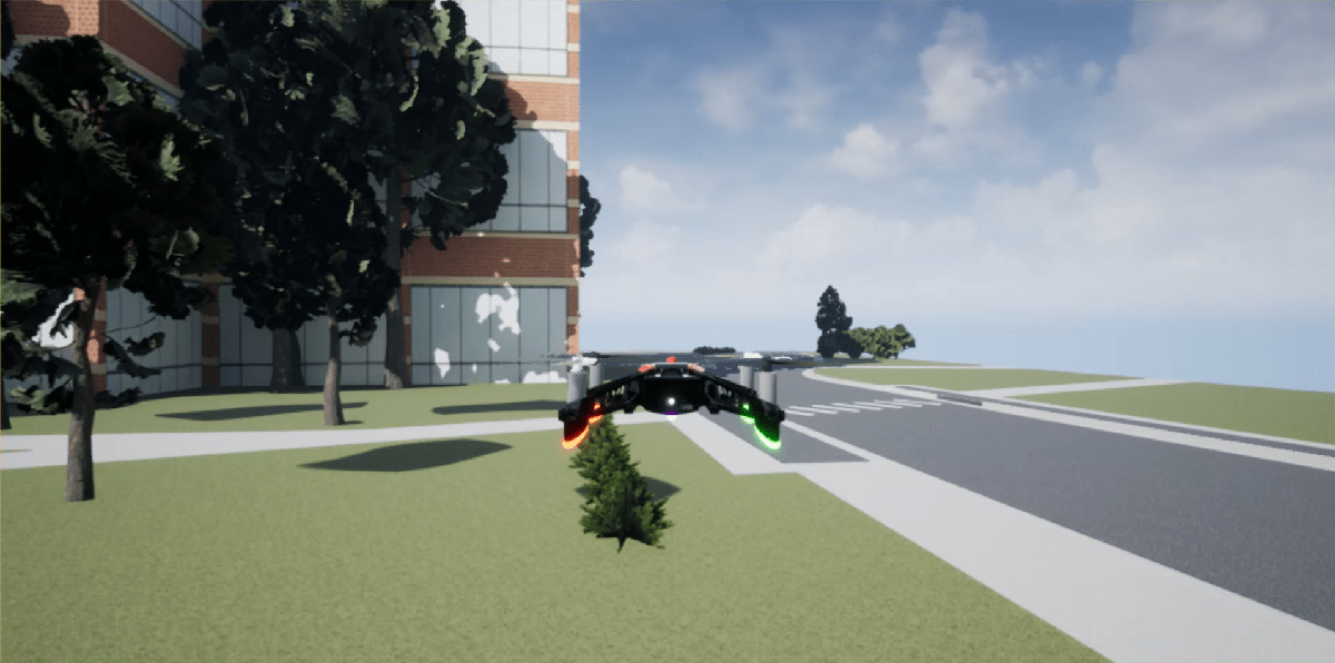
AppleHill scene: requires Unreal from Epic Games® and the Aerospace Blockset Interface for Unreal Engine® support package installed.

Implementation

The AC cmd bus signal from the Command subsystem forms the reference signal to the FCS subsystem.
The Environment bus signal from the Environment subsystem has the environment data and is passed on to the Sensors subsystem (acceleration due to gravity input for the Inertial Measurement Unit), and the Airframe subsystem (used in computation of forces and moments).
The Sensors bus signal and the Image Data from Sensors subsystem form the measured signal, providing information on the current state of vehicle, to the FCS subsystem.
The FCS subsystem consisting of estimators and controllers computes the command signal to the quadcopter motors, Actuators, based on the reference and measured signals. The additional output from FCS, Flag will stop the simulation if the vehicle state values (position and velocity) cross certain safe limits.
The Airframe subsystem acting as the plant model, takes the Actuator commands as inputs to the motors corresponding to the four rotors of the quadcopter. The Multirotor block, the implementation of which is based on [2], and [3], is used in the computation of forces and moments. The output from the Airframe subsystem is the States bus signal, which is fed back to the Sensors subsystem.
The Visualization subsystem uses the AC cmd bus signal(reference command signal), the Actuators input generated by FCS, and the States bus signal from Aiframe subsystem to aid in the visualization.

Trajectory Generation

A trajectory generation tool, using the Dubin method, creates a set of navigational waypoints. To create a trajectory with a set of waypoints this method uses a set of poses defined by position, heading, turn curvature, and turn direction.

To start the tool, ensure that the project is open and run:

asbTrajectoryTool

The following interface displays:

The interface has several panels:

Waypoints

This panel describes the poses the trajectory tool requires. To define these poses, the panel uses text boxes:

North and East (position in meters)
Heading (degrees from North)
Curvature (turning curvature in meters^-1)
Turn (direction clockwise or counter-clockwise)

A list of poses appears in the waypoint list to the right of the text boxes.

To add a waypoint, enter pose values in the edit boxes and click Add. The new waypoint appears in the waypoint list in the same panel.

To edit the characteristics of a waypoint, select the waypoint in the list and click Edit. The characteristics of the waypoints display in the edit boxes. Edit the characteristics as desired, then click OK. To cancel the changes click Cancel.

To delete a waypoint, in the waypoint list, select the waypoint and click Delete.

No-Fly Zone

The panel defines the location and characteristics of the no-fly zones. To define the no-fly zone, the panel uses text boxes:

North and East (position in meters)
Radius (distance in meters)
Margin (safety margin in meters)

Use the Add, Delete, Edit, OK, and Cancel buttons in the same way as for the Waypoints panel.

Mapped Trajectory

This panel plots the trajectory over the Apple Hill campus aerial schematic based on the waypoints and no-fly zone characteristics.

To generate the trajectory, add the waypoint and no-fly zone characteristics to the respective panels, then click Generate Trajectory.

To save the trajectory that is currently in your panel, click the Save button. This button only saves your last trajectory.

To load the last saved trajectory, click Load.

To load the default trajectory, press the Load Default button.

To clear the values in the waypoint and no-fly zone panel, click Clear.

The default data contains poses for specific locations at which the toy quadcopter uses its cameras so the pilot on the ground can estimate the height of the snow on the roof. Three no-fly zones were defined for each of the auxiliary power generators, so in case there is a failure in the quadcopter, it does not cause any damage to the campus infrastructure.

When the example generates the trajectory for the default data, the plot should appear as follows:

The red line represents the trajectory, black x markers determine either a change in the trajectory or a specific pose. Blue lines that represent the heading for that specific waypoint accompany specific poses. No-fly zones are represented as green circles.

References

[1] https://github.com/Parrot-Developers/RollingSpiderEdu/tree/master/MIT_MatlabToolbox/trunk/matlab/libs/RoboticsToolbox.

[2] Prouty, R. Helicopter Performance, Stability, and Control. PWS Publishers, 2005.

[3] Pounds, P., Mahony, R., Corke, P. Modelling and control of a large quadrotor robot. Control Engineering Practice. 2010.