mTRF-Toolbox
mTRF-Toolbox is a MATLAB package for modelling multivariate stimulus-response data, suitable for neurophysiological data such as MEG, EEG, sEEG, ECoG and EMG. It can be used to model the functional relationship between neuronal populations and dynamic sensory inputs such as natural scenes and sounds, or build neural decoders for reconstructing stimulus features and developing real-time applications such as brain-computer interfaces (BCIs).
Download and unzip mTRF-Toolbox to a local directory, then in the MATLAB/GNU Octave command window enter:
addpath(genpath('directory/mTRF-Toolbox-2.4/mtrf'))
savepath
Alternatively, use the MATLAB dialog box to install mTRF-Toolbox. On the Home tab, in the Environment section, click Set Path. In the Set Path dialog box, click Add Folder with Subfolders and search for mTRF-Toolbox in your local directory and select the mtrf subfolder.
For documentation and citation, please refer to the mTRF-Toolbox papers:
-
Crosse MJ, Di Liberto GM, Bednar A, Lalor EC (2016) The Multivariate Temporal Response Function (mTRF) Toolbox: A MATLAB Toolbox for Relating Neural Signals to Continuous Stimuli. Frontiers in Human Neuroscience 10:604. https://doi.org/10.3389/fnhum.2016.00604
-
Crosse MJ, Zuk NJ, Di Liberto GM, Nidiffer AR, Molholm S, Lalor EC (2021) Linear Modeling of Neurophysiological Responses to Speech and Other Continuous Stimuli: Methodological Considerations for Applied Research. Frontiers in Neuroscience 15:705621. https://doi.org/10.3389/fnins.2021.705621
For usage, please see the example code provided in the Examples section below, as well the M-files in the examples folder. For detailed usage, please see the help documentation in each of the function headers.
mTRF-Toolbox consists of the following set of functions:
| Function | Description |
|---|---|
| mTRFcrossval() | Cross-validation for encoding/decoding model optimization |
| mTRFtrain() | Fits an encoding/decoding model (TRF/STRF estimation) |
| mTRFtransform() | Transforms a decoding model into an encoding model |
| mTRFpredict() | Predicts the output of an encoding/decoding model |
| mTRFevaluate() | Evaluates encoding/decoding model performance |
| Function | Description |
|---|---|
| mTRFattncrossval() | Cross-validation for attention decoder optimization |
| mTRFattnevaluate() | Evaluates attention decoder performance |
| mTRFmulticrossval() | Cross-validation for additive multisensory model optimization |
| mTRFmultitrain() | Fits an additive multisensory model (TRF/STRF estimation) |
| Function | Description |
|---|---|
| mTRFenvelope() | Computes the temporal envelope of a continuous signal |
| mTRFresample() | Resamples and smooths temporal features |
| lagGen() | Generates time-lagged input features of multivariate data |
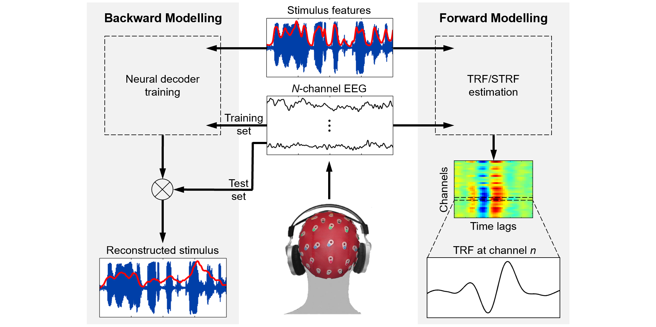
mTRF-Toolbox provides a complementary forward/backward quantitative modelling framework. A forward model, known as a temporal response function or temporal receptive field (TRF), describes how sensory information is encoded in neuronal activity as a function of time (or some other variable). Multivariate stimulus features such as spatio- or spectro-temporal representations, as well as categorical features such as phonetic or semantic embeddings, can be used as inputs to the model. TRFs can be subjected to conventional time-frequency / source analysis techniques, or used to predict the neural responses to an independent set of stimuli. mTRF-Toolbox provides an efficient cross-validation procedure for hyperparameter optimization.
A backward model, known as a neural decoder, treats the direction of causality as if it were in reverse, mapping from the neural response back to the stimulus. Neural decoders can be used to reconstruct stimulus features from information encoded explicitly or implicitly in neuronal activity, or decode higher-order cognitive processes such as selective attention. The mTRF modelling framework provides a basic machine learning platform for real-time BCI applications such as stimulus reconstruction / synthesis and auditory attention decoding (AAD).
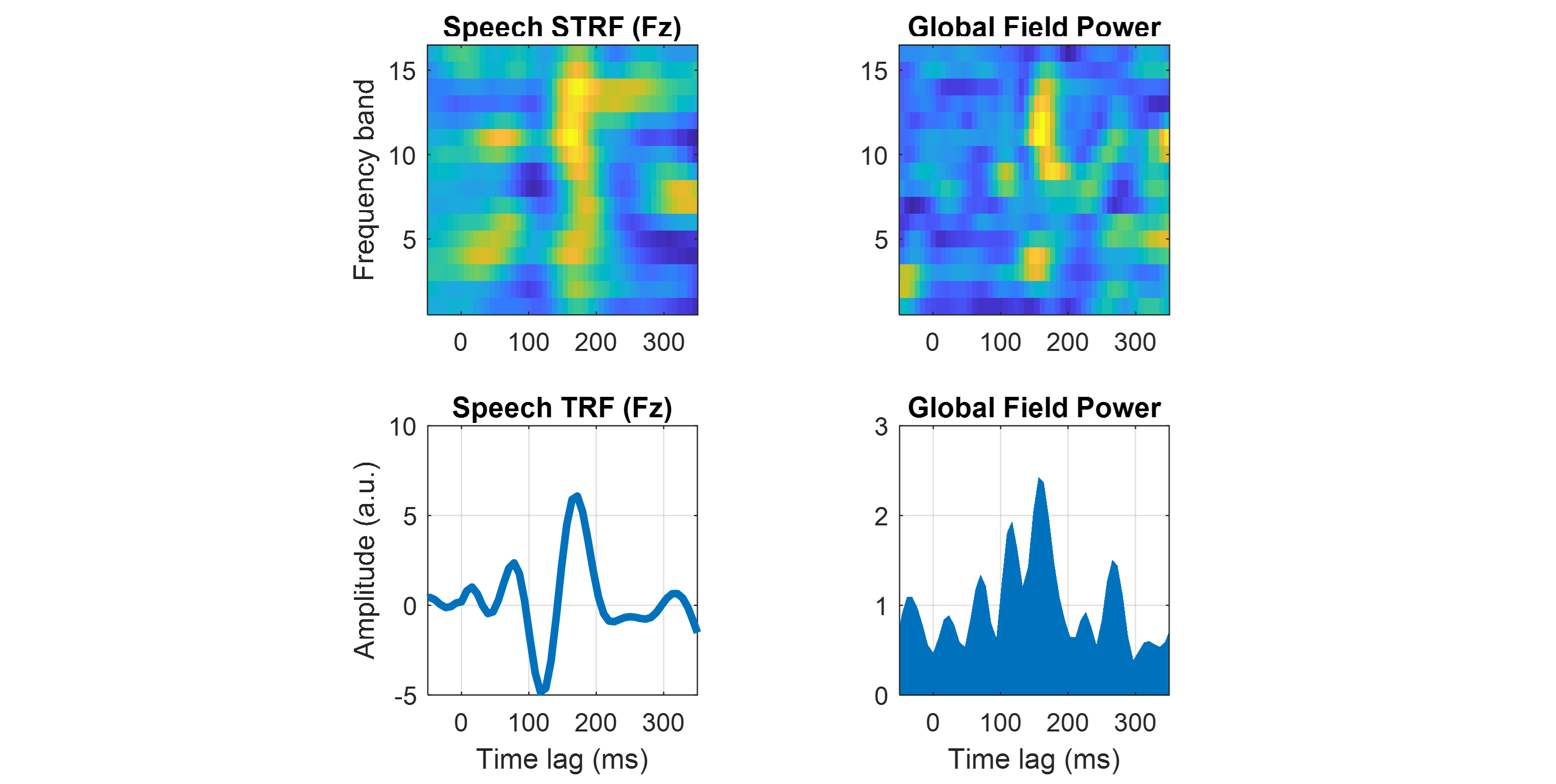
Here, we estimate a 16-channel spectro-temporal response function (STRF) from 2 minutes of EEG data recorded while a human participant listened to natural speech. To map in the forward direction (encoding model), we set the direction of causality to 1. To capture the entire STRF timecourse, the time lags are computed between -100 and 400 ms. The regularization parameter is set to 0.1 to reduce overfitting to noise.
% Load example speech dataset
load('mTRF-Toolbox/data/speech_data.mat','stim','resp','fs','factor');

% Estimate STRF model weights
model = mTRFtrain(stim,resp*factor,fs,1,-100,400,0.1);
We compute the broadband TRF by averaging the STRF model across frequency channels and the global field power (GFP) by taking the standard deviation across EEG channels, and plot them as a function of time lags. This example can also be generated using plot_speech_STRF and plot_speech_TRF.
% Plot STRF
figure
subplot(2,2,1), mTRFplot(model,'mtrf','all',85,[-50,350]);
title('Speech STRF (Fz)'), ylabel('Frequency band'), xlabel('')

% Plot GFP
subplot(2,2,2), mTRFplot(model,'mgfp','all','all',[-50,350]);
title('Global Field Power'), xlabel('')

% Plot TRF
subplot(2,2,3), mTRFplot(model,'trf','all',85,[-50,350]);
title('Speech TRF (Fz)'), ylabel('Amplitude (a.u.)')

% Plot GFP
subplot(2,2,4), mTRFplot(model,'gfp','all','all',[-50,350]);
title('Global Field Power')Here, we build a neural decoder that can reconstruct the envelope of the speech stimulus heard by the EEG participant. First, we downsample the data and partition it into 6 equal segments for training (segments 2 to 6) and testing (segment 1).
% Load data
load('mTRF-Toolbox/data/speech_data.mat','stim','resp','fs');

% Normalize and downsample data
stim = resample(sum(stim,2),64,fs);
resp = resample(resp/std(resp(:)),64,fs);
fs = 64;

% Partition data into training/test sets
nfold = 6; testTrial = 1;
[strain,rtrain,stest,rtest] = mTRFpartition(stim,resp,nfold,testTrial);
To optimize the decoders ability to predict stimulus features from new EEG data, we tune the regularization parameter using an efficient leave-one-out cross-validation (CV) procedure.
% Model hyperparameters
Dir = -1; % direction of causality
tmin = 0; % minimum time lag (ms)
tmax = 250; % maximum time lag (ms)
lambda = 10.^(-6:2:6); % regularization parameters

% Run efficient cross-validation
cv = mTRFcrossval(strain,rtrain,fs,Dir,tmin,tmax,lambda,'zeropad',0,'fast',1);
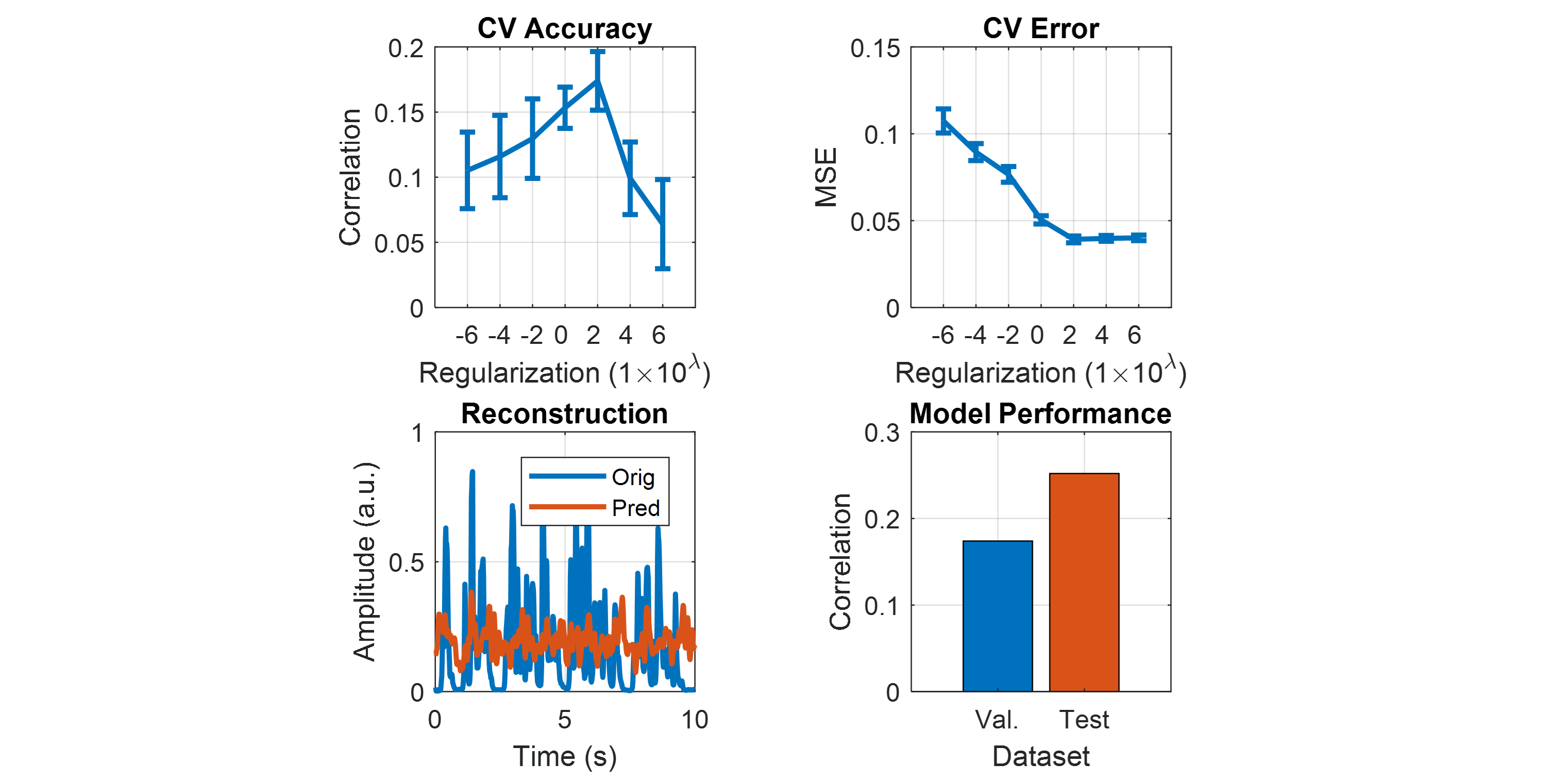
Based on the CV results, we train our model using the optimal regularization value and test it on the held-out test set. Model performance is evaluated by measuring the correlation between the original and predicted stimulus.
% Find optimal regularization value
[rmax,idx] = max(mean(cv.r));

% Train model
model = mTRFtrain(strain,rtrain,fs,Dir,tmin,tmax,lambda(idx),'zeropad',0);

% Test model
[pred,test] = mTRFpredict(stest,rtest,model,'zeropad',0);
We plot the CV metrics as a function of regularization and the test results of the final model. This example can also be generated using stimulus_reconstruction.
% Plot CV accuracy
figure
subplot(2,2,1), errorbar(1:numel(lambda),mean(cv.r),std(cv.r)/sqrt(nfold-1),'linewidth',2)
set(gca,'xtick',1:nlambda,'xticklabel',-6:2:6), xlim([0,numel(lambda)+1]), axis square, grid on
title('CV Accuracy'), xlabel('Regularization (1\times10^\lambda)'), ylabel('Correlation')

% Plot CV error
subplot(2,2,2), errorbar(1:numel(lambda),mean(cv.err),std(cv.err)/sqrt(nfold-1),'linewidth',2)
set(gca,'xtick',1:nlambda,'xticklabel',-6:2:6), xlim([0,numel(lambda)+1]), axis square, grid on
title('CV Error'), xlabel('Regularization (1\times10^\lambda)'), ylabel('MSE')

% Plot reconstruction
subplot(2,2,3), plot((1:length(stest))/fs,stest,'linewidth',2), hold on
plot((1:length(pred))/fs,pred,'linewidth',2), hold off, xlim([0,10]), axis square, grid on
title('Reconstruction'), xlabel('Time (s)'), ylabel('Amplitude (a.u.)'), legend('Orig','Pred')

% Plot test accuracy
subplot(2,2,4), bar(1,rmax), hold on, bar(2,test.r), hold off
set(gca,'xtick',1:2,'xticklabel',{'Val.','Test'}), axis square, grid on
title('Model Performance'), xlabel('Dataset'), ylabel('Correlation')Here, we evaluate the contribution of individual time lags towards stimulus reconstruction using a single-lag decoder analysis. First, we downsample the data and partition it into 5 equal segments.
% Load data
load('mTRF-Toolbox/data/speech_data.mat','stim','resp','fs');

% Normalize and downsample data
stim = resample(sum(stim,2),64,fs);
resp = resample(resp/std(resp(:)),64,fs);
fs = 64;

% Generate training/test sets
nfold = 10;
[strain,rtrain] = mTRFpartition(stim,resp,nfold);
We run a leave-one-out cross-validation to test a series of single-lag decoders over the range 0 to 1000 ms using a pre-tuned regularization parameter.
% Run single-lag cross-validation
[stats,t] = mTRFcrossval(strain,rtrain,fs,-1,0,1e3,10.^-2,'type','single','zeropad',0);

% Compute mean and variance
macc = squeeze(mean(stats.r))'; vacc = squeeze(var(stats.r))';
merr = squeeze(mean(stats.err))'; verr = squeeze(var(stats.err))';

% Compute variance bound
xacc = [-fliplr(t),-t]; yacc = [fliplr(macc-sqrt(vacc/nfold)),macc+sqrt(vacc/nfold)];
xerr = [-fliplr(t),-t]; yerr = [fliplr(merr-sqrt(verr/nfold)),merr+sqrt(verr/nfold)];
We plot the reconstruction accuracy and error as a function of time lags. This example can also be generated using single_lag_analysis.
% Plot accuracy
figure
subplot(1,2,1), h = fill(xacc,yacc,'b','edgecolor','none'); hold on
set(h,'facealpha',0.2), xlim([tmin,tmax]), axis square, grid on
plot(-fliplr(t),fliplr(macc),'linewidth',2), hold off
title('Reconstruction Accuracy'), xlabel('Time lag (ms)'), ylabel('Correlation')

% Plot error
subplot(1,2,2)
h = fill(xerr,yerr,'b','edgecolor','none'); hold on
set(h,'facealpha',0.2), xlim([tmin,tmax]), axis square, grid on
plot(-fliplr(t),fliplr(merr),'linewidth',2), hold off
title('Reconstruction Error'), xlabel('Time lag (ms)'), ylabel('MSE')If you publish any work using mTRF-Toolbox, please it cite as:
Crosse MJ, Di Liberto GM, Bednar A, Lalor EC (2016) The Multivariate Temporal Response Function (mTRF) Toolbox: A MATLAB Toolbox for Relating Neural Signals to Continuous Stimuli. Frontiers in Human Neuroscience 10:604.
@article{crosse2016mtrf,
  title={The multivariate temporal response function (mTRF) toolbox: a MATLAB toolbox for relating neural signals to continuous stimuli},
  author={Crosse, Michael J and Di Liberto, Giovanni M and Bednar, Adam and Lalor, Edmund C},
  journal={Frontiers in Human Neuroscience},
  volume={10},
  pages={604},
  year={2016},
  publisher={Frontiers}
}
Zitieren als
Crosse, Michael J., et al. “The Multivariate Temporal Response Function (MTRF) Toolbox: A MATLAB Toolbox for Relating Neural Signals to Continuous Stimuli.” Frontiers in Human Neuroscience, vol. 10, Frontiers Media SA, Nov. 2016, doi:10.3389/fnhum.2016.00604.
Crosse, Michael J., et al. “Linear Modeling of Neurophysiological Responses to Speech and Other Continuous Stimuli: Methodological Considerations for Applied Research.” Frontiers in Neuroscience, vol. 15, Frontiers Media SA, Nov. 2021, doi:10.3389/fnins.2021.705621.
Kompatibilität der MATLAB-Version
Plattform-Kompatibilität
Windows macOS LinuxKategorien
- AI, Data Science, and Statistics > Statistics and Machine Learning Toolbox >
- Sciences > Neuroscience > Brain Computer Interfaces >
- Engineering > Biomedical Engineering > Biomedical Signal Processing >
Tags
Community Treasure Hunt
Find the treasures in MATLAB Central and discover how the community can help you!
Start Hunting!Live Editor erkunden
Erstellen Sie Skripte mit Code, Ausgabe und formatiertem Text in einem einzigen ausführbaren Dokument.
examples
mtrf
Versionen, die den GitHub-Standardzweig verwenden, können nicht heruntergeladen werden
| Version | Veröffentlicht | Versionshinweise | |
|---|---|---|---|
| 2.4 | See release notes for this release on GitHub: https://github.com/mickcrosse/mTRF-Toolbox/releases/tag/v2.4 |
||
| 2.3 | The following updates were made to v2.3: 1. Fixed correlation broadcasting issue for older versions
Thanks to Maya Kaufman for flagging the above issues. |
|
|
| 2.2 | The following updates were made to v2.2: 1. Fixed MSE input argument bug
|
|
|
| 2.1 | The following updates were made to v2.1:
|
|
|
| 2.0.3 | Added function for CV data partitioning, added feature for equal fold generation, changed AMI metric to ADI metric for attention decoder optimization, added feature for specifying evaluation metrics. |
|
|
| 2.0.2 | New structuring of toolbox, new functions and features, new example scripts, faster and memory-efficient cross-validation, no additional MathWorks toolboxes required. |
|
|
| 2.0.1 | * Migrated parsevarargin within main functions
|
|
|
| 2.0.0 |
|


