Results for

New to r2020a, leapseconds() creates a table showing all leap seconds recognized by the datetime data type.

>> leapseconds()
ans =
  27×2 timetable
       Date        Type    CumulativeAdjustment
    ___________    ____    ____________________
    30-Jun-1972     +              1 sec       
    31-Dec-1972     +              2 sec       
    31-Dec-1973     +              3 sec       
    31-Dec-1974     +              4 sec       
    31-Dec-1975     +              5 sec       
             << 21 rows removed >>
    31-Dec-2016     +             27 sec   

Leap seconds can covertly sneak into your data and cause errors that are difficult to resolve if the leap seconds go undetected. A leap second was responsible for crashing Reddit , Mozilla, Yelp, LinkedIn and other sites in 2012.

Detect leap seconds present in a vector of years

% Define a vector of years
t = 2005:2008; 

allLeapSeconds = leapseconds(); 
isYearWithLeapSecond = ismember(t,year(allLeapSeconds.Date));

% Show years that contain a leap second
t(isYearWithLeapSecond)
ans =
        2005        2008

Detect leap seconds present in a vector of months

% Define a vector of months 
t = datetime(1972, 1, 1) + calmonths(0:11);

t.Format = 'MMM-yyyy';
allLeapSeconds = leapseconds(); 
[tY,tM] = ymd(t); 
[leapSecY, leapSecM] = ymd(allLeapSeconds.Date); 
isMonthWithLeapSecond = ismember([tY(:),tM(:)], [leapSecY, leapSecM], 'rows');

% Show months that contain a leap second
t(isMonthWithLeapSecond)
ans = 
  1×2 datetime array
   Jun-1972   Dec-1972

List all leap seconds in your lifetime

% Enter your birthday in mm/dd/yyyy hh:mm:ss format
yourBirthday = '01/15/1988 14:30:00'; 

yourTimeRange = timerange(datetime(yourBirthday), datetime('now')); 
allLeapSeconds = leapseconds(); 
lifeLeapSeconds = allLeapSeconds(yourTimeRange,:);
lifeLeapSeconds.YourAge = lifeLeapSeconds.Date - datetime(yourBirthday);
lifeLeapSeconds.YourAge.Format = 'y';

% Show table
fprintf('\n Leap seconds in your lifetime:\n')
disp(lifeLeapSeconds)

Leap seconds in your lifetime:
       Date        Type    CumulativeAdjustment     YourAge  
    ___________    ____    ____________________    __________
    31-Dec-1989     +             15 sec           1.9587 yrs
    31-Dec-1990     +             16 sec            2.958 yrs
                        << 8 rows removed >>
    30-Jun-2012     +             25 sec           24.456 yrs
    30-Jun-2015     +             26 sec           27.454 yrs
    31-Dec-2016     +             27 sec            28.96 yrs

What is a leap second?

A second is defined as the time it takes a cesium-133 atom to oscillate 9,192,631,770 times under controlled conditions. The transition frequency is so precise that it takes 100 million years to gain 1 second of error [1]. If the earth’s rotation were perfectly synchronized to the atomic second, a day would be 86,400 seconds. But the earth’s rate of rotation is affected by climate, winds, atmospheric pressure, and the rate of rotation is gradually decreasing due to tidal friction [2,3]. Several months before the expected difference between the atomic clock-based time (UTC) and universal time (UT1) reaches +/- 0.9 seconds the IERS authorizes the addition (or subtraction) of 1 leap second (see plot below). Since the first leap second in 1972, all leap second adjustments have been made on the last day of June or December and all adjustments have been +1 second which explains the + signs in the type column of the leapseconds() table.

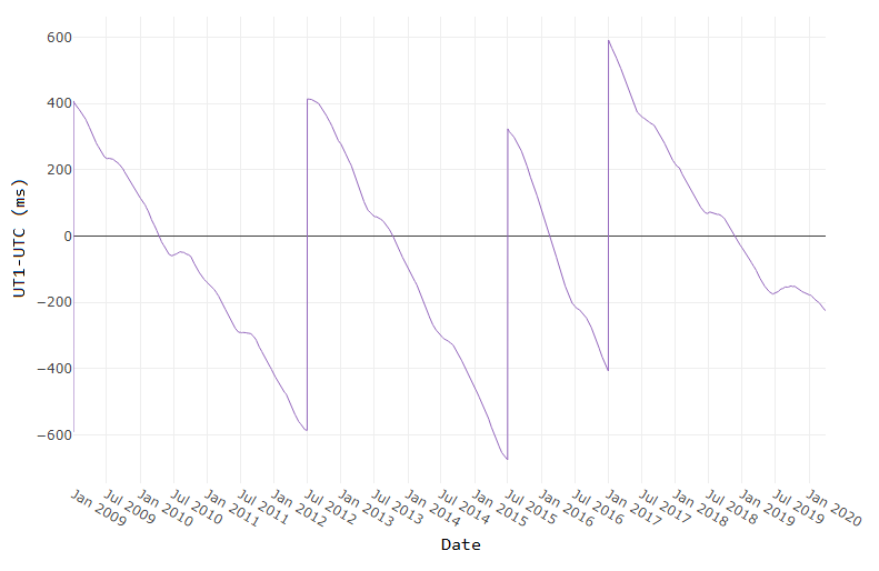
[ Image source ]

How to reference the leap second schedule in your code

Since leap second adjustments are not regularly timed, you can record the official IERS Bulletin C version used at the time of your analysis by accessing the 2nd output to leapseconds().

[T,vers] = leapseconds

What do leap seconds look like in datetime values?

A minute typically has 60 seconds spanning from 0:59. A minute containing a leap second has 61 seconds spanning from 0:60.

December 30, 2016 was a normal day. If we add the usual 86400 seconds to the start of that day, the result is the start of the next day.

d = datetime(2016, 12, 30, 'TimeZone','UTCLeapSeconds') + seconds(86400)
d = 
  datetime
   2016-12-31T00:00:00.000Z

The next day, December 31, 2016, had a leap second. If we add 86400 seconds to the start of that day, the result is not the start of the next day.

d = datetime(2016, 12, 31, 'TimeZone','UTCLeapSeconds') + seconds(86400)
d = 
  datetime
   2016-12-31T23:59:60.000Z

When will the next leap second be?

As of the current date (April 2020) the timing of the next leap second is unknown. Based on the data from the plot above, what's your guess?

References

1. https://www.timeanddate.com/time/how-do-atomic-clocks-work.html
2. https://www.nasa.gov/centers/goddard/news/topstory/2003/0210rotation.html
3. https://en.wikipedia.org/wiki/%CE%94T#Universal_time

Do date ranges from two different timetables intersect?

Is a specific datetime value within the range of a timetable?

Is the range of row times in a timetable within the limits of a datetime array?

Three new functions in r2020a will help to answer these questions.

• [tf, whichRows] = containsrange(TT,__)
• [tf, whichRows] = overlapsrange(TT,__)
• [tf, whichRows] = withinrange(TT,__)

In these function inputs, TT is a timetable and input #2 is one of the following:

• another timetable
• a time range object produced by timerange(startTime,endTime)
• a datetime scalar produced by datetime()
• a duration

The tf output is a logical scalar indicating pass|fail and the whichRows output is a logical vector identifying the rows of TT that are within the specified time range.

How do these functions differ?

Let's test all 3 functions with different time ranges and a timetable of electric utility outages in the United States, provided by Matlab. The first few rows of outages.csv are shown below in a timetable. You can see that the row times are not sorted which won't affect the behavior of these functions.

8×5 timetable
     OutageTime          Region         Loss     Customers     RestorationTime            Cause       
  ________________    _____________    ______    __________    ________________    ___________________
  2002-02-01 12:18    {'SouthWest'}    458.98    1.8202e+06    2002-02-07 16:50    {'winter storm'   }
  2003-01-23 00:49    {'SouthEast'}    530.14    2.1204e+05                 NaT    {'winter storm'   }
  2003-02-07 21:15    {'SouthEast'}     289.4    1.4294e+05    2003-02-17 08:14    {'winter storm'   }
  2004-04-06 05:44    {'West'     }    434.81    3.4037e+05    2004-04-06 06:10    {'equipment fault'}
  2002-03-16 06:18    {'MidWest'  }    186.44    2.1275e+05    2002-03-18 23:23    {'severe storm'   }
  2003-06-18 02:49    {'West'     }         0             0    2003-06-18 10:54    {'attack'         }
  2004-06-20 14:39    {'West'     }    231.29           NaN    2004-06-20 19:16    {'equipment fault'}
  2002-06-06 19:28    {'West'     }    311.86           NaN    2002-06-07 00:51    {'equipment fault'}

The range of times in utility.csv is depicted by the gray timeline bar in the plot below labeled "Timetable row times". The timeline bars above it are various time ranges or scalar datetime values used to test the three new functions.

The three columns of checkboxes on the right of the plot show the results of the first output of each function, tf, for each time range.

The time ranges were created by the timerange function using the syntax timerange(startTime,endTime). The default intervalType in timerange() is 'openright' which means that datetimes are matched when they are equal to or greater than startTime and less than but not equal to endTime. The scalar datetime values were created with datetime().

The colorbar along with the colored points at the bottom of each timeline bar show the row numbers of timetable TT that were selected by the whichRows output of the three functions.

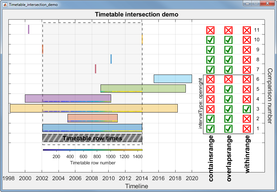
The containsrange() function returns true when all of the time range values are within the timetable including the timetable's minimum and maximum datetime.

The overlapsrange() function returns true when any of the time range values are with the timetable's range.

The withinrange() function returns true only when all of the timetable's datetime values are within the time range values. A careful observer may see that comparison number 1 is false even though that time range is exactly equal to the timetable's row time range. This is because the default value for intervalType in the timerange() function is 'openright' which does not match the end values if they are equal. If you change the intervalType to 'closed' the withinrange result for comparison 1 would be true.

The scalar datetime values for comparisons 8, 9 and 10 are all exact matches of datetimes within the timetable and result in a single match in the whichRows output. The datetime values for comparisons 7 and 11 do not match any of the timetable row times and the values in whichRows are all false even though comparison 7 is within the timetable range. For all three tests, the whichRows outputs are identical.

---------------------------------------------------------------

Here is the code used to generate this data, test the functions, and produce the plot.

% Read in the outage data as a table and convert it to a timetable TT.
T = readtable('outages.csv');
TT = table2timetable(T);

% Look at the first few rows.
head(TT)
% Show that row time vector is not sorted.
issorted(TT)

% Get the earliest and latest row time.
outageTimeLims = [min(TT.OutageTime), max(TT.OutageTime)];

% Define time ranges to test [start,end] or scalar times [datetime, NaT]
% The scalar times must be listed after time ranges.
dateRanges = [ % start, end
    outageTimeLims;                                 % original data
    outageTimeLims;                                 % equal time range
    datetime(2005,2,1), datetime(2011,2,1);         % all within
    datetime(1998,3,16), datetime(2018,4,11);       % starts before, ends after
    datetime(2000,1,1), datetime(2010,4,11);        % starts before, ends within
    datetime(2009,1,15), datetime(2019, 4,7);       % starts within, ends after
    datetime(2015,6,15), datetime(2019,12,31);      % all outside
    datetime(2008,6,6), NaT;                        % 1-value, inside, not a member
    [TT.OutageTime(find(year(TT.OutageTime)==2010,1)), NaT] % 1 value, inside, is a member
    outageTimeLims(1), NaT;                         % 1-value, on left edge
    outageTimeLims(2), NaT;                         % 1-value, on right edge
    datetime(2000,6,6), NaT;                        % 1-value, outside
    ];
nRanges = size(dateRanges,1);
dateRangeLims = [min(dateRanges,[],'all'), max(dateRanges,[],'all')];

% Set up the figure and axes
uifig = uifigure('Name', 'Timetable_intersection_demo', 'Resize', 'off');
uifig.Position(3:4) = [874,580];
movegui(uifig,'center')
uiax = uiaxes(uifig, 'Position', [0,0,uifig.Position(3:4)], 'box', 'on', 'YAxisLocation', 'right',...
    'ytick', -.5:1:nRanges, 'YTickLabel', [], 'ylim', [-3.5, nRanges], 'FontSize', 18);
hold(uiax, 'on')
grid(uiax, 'on')
uiax.Toolbar.Visible = 'off';
% Add axes labels & title
title(uiax, strrep(uifig.Name,'_',' '))
xlabel(uiax, 'Timeline')
ylab = ylabel(uiax, 'Comparison number');
set(ylab, 'Rotation', -90, 'VerticalAlignment', 'Bottom')

% Add the timetable frame
fill(uiax, outageTimeLims([1,2,2,1]), [-.7,-.7,nRanges-.3,nRanges-.3] , 0.85938*[1,1,1], ... %gainsboro
    'EdgeColor', 0.41016*[1,1,1], 'LineStyle', '--', 'LineWidth', 1.5, 'FaceAlpha', .25)     %dimgray

% Set xtick & xlim after x-axis is converted to datetime
range = @(x)max(x)-min(x); 
uiax.XLim = dateRangeLims + range(dateRangeLims).*[-.01, .40];
uiax.XTick = dateshift(dateRangeLims(1),'start','Year') : calyears(2) : dateshift(dateRangeLims(2),'start','Year','next');
xtickformat(uiax,'yyyy')

% Set up timeline plot
lineColors = [0.41016*[1,1,1]; lines(nRanges-1)]; %dimGray
uiax.Colormap = parula(size(TT,1));
tfUniCodes = {char(09745),char(09746)}; %{true, false} checkbox characters
barHeight = 0.8;
rightMargin = [max(dateRangeLims),max(uiax.XLim)];
tfCenters = linspace(rightMargin(1),rightMargin(2),5);
tfCenters([1,end]) = [];
intervalType = 'openright';  % open, closed, openleft openright(def);  see https://www.mathworks.com/help/matlab/ref/timerange.html#bvdk6vh-intervalType

% Loop through each row of dateRanges
for i = 0:nRanges-1
    % Plot timeline bar
    pObj = fill(uiax, dateRanges(i+1,[1,2,2,1]), i+[-barHeight,-barHeight,barHeight,barHeight]/2, lineColors(i+1,:), 'FaceAlpha', .4);

      % Evaluate date ranges and single values differently
      if any(isnat(dateRanges(i+1,:)))
          % Test single datetime
          tr = dateRanges(i+1,~isnat(dateRanges(i+1,:)));
          set(pObj, 'LineWidth', 3, 'EdgeAlpha', .6, 'EdgeColor', lineColors(i+1,:))
      else
          % Test date range
          tr = timerange(dateRanges(i+1,1), dateRanges(i+1,2),intervalType);
      end

      % Create timerange obj and test for intersections
      [tf(1), whichRows{1}] = containsrange(TT,tr);
      [tf(2), whichRows{2}] = overlapsrange(TT,tr);
      [tf(3), whichRows{3}] = withinrange(TT,tr);
      % Confirm that all 'whichRows' are equal
      assert(isequal(whichRows{1},whichRows{2},whichRows{3}), 'Unequal whichRows outputs.')

      if i>0
          % Add pass/fail checkboxes
          text(uiax, tfCenters(tf), repmat(i,1,sum(tf)), repmat(tfUniCodes(1),1,sum(tf)), ...
              'HorizontalAlignment', 'Center', 'Color', [0 .5 0], 'FontSize', 36, 'FontWeight', 'Bold')
          % Fail checkboxes
          text(uiax, tfCenters(~tf), repmat(i,1,sum(~tf)), repmat(tfUniCodes(2),1,sum(~tf)), ...
              'HorizontalAlignment', 'Center', 'Color', [1 0 0], 'FontSize', 36, 'FontWeight', 'Bold')

          % Plot the TT row number matches
          scatter(uiax, TT.OutageTime(whichRows{1}), repmat(i-barHeight/2+.1,1,sum(whichRows{1})), ...
              10, uiax.Colormap(whichRows{1},:), 'filled', 'MarkerFaceAlpha', 0.2)
      else
          % add stripes to reference bar
          xHatch = linspace(dateRanges(i+1,1)-days(2), dateRanges(i+1,2)+days(2), 20);
          yHatch = repmat(unique(pObj.YData), 1, 19);
          plot(uiax, [xHatch(1:end-1);xHatch(2:end)], yHatch, '-', 'Color', [1 1 1 .5], 'LineWidth', 4)
          pObj.FaceAlpha = .9;
          text(uiax, mean(outageTimeLims), 0, 'Timetable row times', 'FontSize', 20, ...
              'HorizontalAlignment', 'Center', 'VerticalAlignment', 'middle', 'FontWeight', 'Bold')
      end
  end

% Draw frame around checkboxs for duration comparisons and label intervalType
rectEdges = linspace(rightMargin(1),rightMargin(2),33);
nDurations = sum(~isnat(dateRanges(:,2)))-1;
fill(uiax, rectEdges([6,end-5,end-5,6]), [.4 .4 nDurations+[.4,.4]], 'w', ...
    'FaceAlpha', 0, 'LineWidth', 1.5, 'EdgeColor', 0.41016*[1,1,1]) % dimgray
text(uiax, rectEdges(6), nDurations/2+.5, sprintf('intervalType: %s', intervalType), 'FontSize', 16, ...
    'HorizontalAlignment', 'Center', 'VerticalAlignment', 'Bottom', 'Rotation', 90)

% Add text labels for checkboxes and comparison number
text(uiax, tfCenters, [.5 .5 .5], {'containsrange ', 'overlapsrange ', 'withinrange '}, 'Fontsize', 22, 'Rotation', 90, ...
    'HorizontalAlignment', 'right', 'FontWeight', 'b')
text(uiax, repmat(rightMargin(2)-range(xlim(uiax))*.02,1,nRanges-1), 1:nRanges-1, cellstr(num2str((1:nRanges-1)')), ...
    'HorizontalAlignment', 'Right', 'FontSize', 16)

% Add color bar; position it under the timetable bar (must be done after all other axes properties are set)
% requires coordinate tranformation from data units to fig position units.
cb = colorbar(uiax, 'Location', 'South', 'TickDirection', 'Out', 'YAxisLocation', 'Bottom', 'FontSize', 11);
caxis(uiax, [1,size(TT,1)])
cb.Position(3) = range(outageTimeLims)/range(xlim(uiax))  * (uiax.InnerPosition(3)/uifig.Position(3));
cb.Position(1) = ((outageTimeLims(1)-min(xlim(uiax)))/range(xlim(uiax)) * uiax.InnerPosition(3) + uiax.InnerPosition(1)) / uifig.Position(3); 
cb.Position(4) = 0.008;
cb.Position(2) = ((-barHeight-min(ylim(uiax))-.5)/range(ylim(uiax)) * uiax.InnerPosition(4) + uiax.InnerPosition(2)) / uifig.Position(4);
ylabel(cb, 'Timetable row number')

The following is a list of updates and new features for File Exchange and Cody.

New Features

• (Coming soon) Support for GitHub releases added to File Exchange - Stay tuned for an upcoming announcement later this month.

• 2 new Cody problem groups - Visit Cody to see the new MATLAB Basics and Beyond the Basics problem groups.

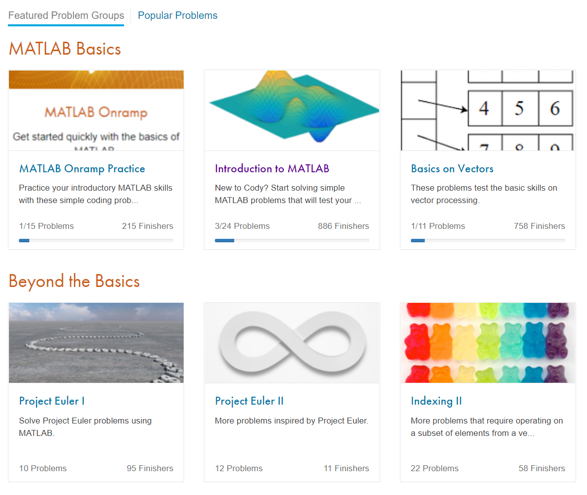
Let us know what you think about these new features by replying below.

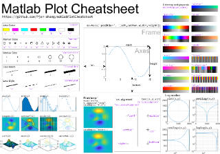
Take a look at this handy cheatsheet from Peijin Zhang, a PhD student of solar radio at USTC, China. This is especially helpful for those preparing figures for a paper.

https://github.com/Pjer-zhang/matlabPlotCheatsheet

Do you know of any other cheatsheets for MATLAB?

Cody has a wealth of problem groups that allow users of various skill levels to improve programming skills vis-à-vis MATLAB in an engaging way.

I would like to highlight the Draw Letters group, composed of problems created by Majid Farzaneh.

If you haven't yet visited Cody or solved that problem group, I would recommend that you head over there now. What are you waiting for?

We have created a new distance learning community for educators who are teaching remotely or online using MathWorks tools. It houses resources, such as articles, code examples, and videos, as well as an area where community members can ask questions or hold discussions around best practices in distance learning. Jiro Doke , who also writes for the File Exchange Pick of the Week blog, will be moderating this community.

We encourage you to visit the new community and share best practices, examples, and ask questions.

We have created a new page in MATLAB Answers that aggregates the most frequently asked MATLAB questions (FAQs). FAQs are common and a good starting point for anyone learning something new and having them all in one place can be a useful resource. Our new FAQ page lists the top 100 MATLAB questions asked and answered in MATLAB Central . They are grouped into the following 9 categories:

• Data Import and Analysis
• Graphics: Basics
• Graphics: Objects
• Installation and Licensing
• Language Fundamentals: Basics
• Language Fundamentals: Matrices and Arrays
• Language Fundamentals: Operators and Elementary Operations
• Mathematics
• Programming

I recommend that everyone scans the new FAQ page as you might find some useful tips.

We will be updating the FAQ page regularly as new questions are asked in the community. We welcome any feedback you have.

Check out this pick of the week from Emma Gau. Emma's submission is featured on the Live Script gallery. Check out the blog post to see why Owen picked it.

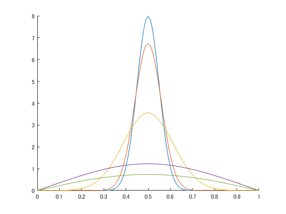
Check out this pick of the week from Will. Steve's progressbar submission has been around since 2005 and still runs perfectly. Check out the blog post to see why Will picked it.

We are excited to announce that Adam Danz has accepted our invitation and now is a member of the Community Advisory Board (CAB)!

Adam has been a rising star in Answers, obtaining 4500+ reputation points in the past year! Furthermore, he has contributed high-quality files to File Exchange, with an average rating of 4.8. Adam also demonstrates good communication skills and the ability to work with others. Those characteristics are what we expect to see from a CAB advisor. You can learn more about him and CAB on the CAB page .

On behalf of all the community team, we would like to extend our warmest welcome to Adam!

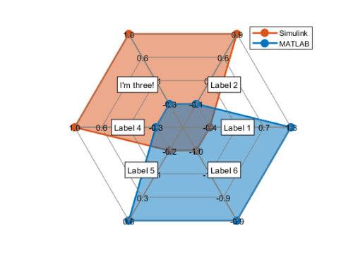
Check out Sean's blog posts ( Intro , Authoring ) on Spider Plots. He's using spider_plot by Moses to create beautiful plots like this.

The following is a list of updates and new features for MATLAB Central, including MATLAB Answers, File Exchange, Blogs, and Cody.

New Features

Community highlights channel released - See this post for more details.

Answers comment UI change - A minor improvement to the user interface when adding comments to questions and answers in MATLAB Answers. This change should make it easier to discern between commenting and adding a new answers to a question.

Answers rich text editor update - The rich text editor has been updated to the 19b version of the MATLAB Live Editor. This update will primarily help with syntax highlighting along with resolving a few other issues.

Answer pages translation option - Answers translations options added. A translation option for questions and answers content has been added for French, German, Italian, Spanish, and Chinese languages.

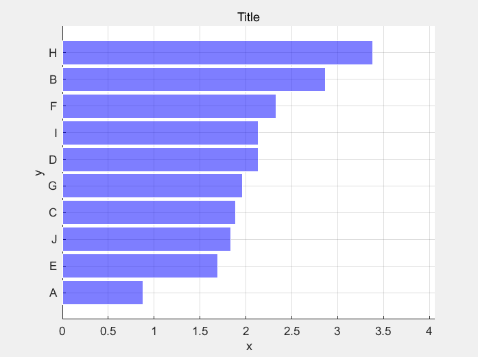
Hey everyone! I'm spotlighting Nikolaos Nikolaou today because of the sheer quantity of his Cody solutions over such a relatively short time span. Nikolaos has submitted 1,161 Cody solutions over the last 6 months of 2019, averaging 6.4 solutions per day. Achieving a Cody rank of 19 with a score of 18,820 and earning him a plethora of badges (including the Speed Demon badge of course). He's completed 24 problem groups and is well into most of the remaining 35.

Way to go Nikolaos!

Check out digCircs by Graham W Griffiths, this weeks pick by Sean . Read Sean's blog post about why he picked Graham's submission this week.

Please post any comments to Seans's blog post here.

Check out nextname by Stephen Cobeldick, this weeks pick by Jiro. Read Jiro's blog post about why he picked Stephen's submission this week.

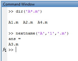
Please post any comments to Jiro's blog post here.

I'm please to announce this new MATLAB Central feature for posting community highlights. This new channel will:

• Allow MathWorks and the community leaders to easily post newsworthy items to the community
• Allow community visitors to respond to these posts with Likes and Replies
• Allow anyone to follow/subscribe the channel so they can be notified of new posts

What do we mean by newsworthy?  In short, this means anything we think some or all of the community might like to know. Here are some examples of what we’re thinking about posting to this new channel.

• New or upcoming community features or events
• User highlights (e.g. examples of good behavior, interesting posts)
• Interesting content (e.g. File Exchange pick of the week submissions)
• Release notes and new features
• Polls (future)

New highlights will appear on the community home page at the time they are posted and all past highlights can be found by going to the community home page and clicking the Highlights link in the right column.

As always, let us know what you think by liking this post or commenting below.

The following is a list of updates and new features for MATLAB Central, including MATLAB Answers, File Exchange, Blogs, and Cody.

New Features

Profile search - A global community profile search has been added. The search field on community profile pages has been updated from a standard content search to a user profile search. This improvement makes it easier to find community members across all MATLAB Central. Previously one had to search the Answers contributors , File Exchange authors , and Cody players page when looking for a user profile.

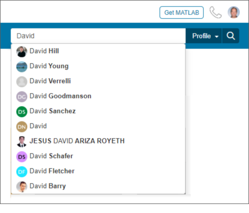
Last seen - We have added a 'last seen' timestamp to community profiles which displays the date of a person's last visit to MATLAB Central. This can be a relevant bit of information and help determine how recent someone has been active in the community.

Answers pages design update - Answers Q&A pages have been updated to remove extra white space. This update includes smaller sized avatars, and position changes for the voting and content actions among other small changes. All these changes also help improve the mobile experience as well.

Original poster styles - Original poster styles have been introduced in Answers. When a question author participates in a Q&A thread their comments or answers will be styled with a blue background and left border so they're easily discernable from other contributors.

File Exchange data in monthly emails - File Exchange stats will be included in the monthly email we send to contributors who've participated in the community on any given month.

Trending content algorithm - The MATLAB Central home page trending content algorithm has been updated to look at content activity over a shorter period of time resulting in a more dynamic feed.