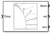
Transform Trajectory

Generate trajectory between two homogeneous transforms

• 

Libraries:
Robotics System Toolbox / Utilities

Description

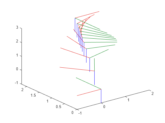
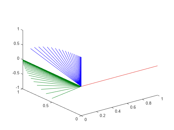
The Transform Trajectory block generates an interpolated trajectory between two homogenous transformation matrices. The block outputs the transform at the times given by the Time input, which can be a scalar or vector.

The trajectory is computed using quaternion spherical linear interpolation (SLERP) for the rotation and linear interpolation for the translation. This method finds the shortest path between positions and rotations of the transformation. Select the Use custom time scaling check box to compute the trajectory using a custom time scaling. The block uses linear time scaling by default.

The initial and final values are held constant outside the time period defined in Time interval.

Examples

Use Custom Time Scaling for Transform Trajectory

Specify custom time-scaling in the Transform Trajectory block to execute an interpolated trajectory. Two transformations are specified in the block to generate a trajectory between the two. The goal is to move between transforms using a nonlinear time scaling where the trajectory moves quickly at the start and slowly at the end.

Open Live Script

Use Custom Time Scaling for a Rotation Trajectory

Specify custom time-scaling in the Rotation Trajectory block to execute an interpolated trajectory. Two rotations are specified in the block to generate a trajectory between them. The goal is to move between rotations using a nonlinear time scaling with more time samples closer to the final rotation.

Open Live Script

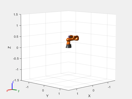
Execute Transformation Trajectory Using Manipulator and Inverse Kinematics

Generate a transformation trajectory using the Transform Trajectory block and execute it for a manipulator robot using inverse kinematics.

Open Live Script

Ports

Input

Time — Time point along trajectory

scalar | vector

Time point along trajectory, specified as a scalar or vector. In general, when specified as a scalar, this value is synced with simulation time and is used to specify the time point for sampling the trajectory. The block outputs a vector of the trajectory variables at that instant in time. If the time is specified as a vector, the block outputs a matrix with each column corresponding to each element of the vector.

Data Types: single | double

T0 — Initial transformation matrix

4-by-4 homogeneous transformation

Initial transformation matrix, specified as a 4-by-4 homogeneous transformation. The function generates a trajectory that starts at the initial orientation, T0, and goes to the final orientation, TF.

Example: trvec2tform([1 10 -1])

Dependencies

To enable this parameter, set the Waypoint source to External.

Data Types: single | double

TF — Final transformation matrix

4-by-4 homogeneous transformation

Final transformation matrix, specified as a 4-by-4 homogeneous transformation. The function generates a trajectory that starts at the initial orientation, T0, and goes to the final orientation, TF.

Example: trvec2tform([1 10 -1])

Dependencies

To enable this parameter, set the Waypoint source to External.

Data Types: single | double

TimeInterval — Start and end times for trajectory

two-element vector

Start and end times for the trajectory, specified as a two-element vector.

Example: [0 10]

Dependencies

To enable this parameter, set the Waypoint source to External.

Data Types: single | double

TSTime — Time scaling time points

scalar | p-element vector

Time scaling time points, specified as a scalar or n p-element vector, where p is the number of points for time scaling. By default, the time scaling is a linear time scaling spanning the TimeInterval. Specify the actual time scaling values in TimeScaling.

If the Time input is specified at a time not specified by these points, interpolation is used to find the right scaling time.

Dependencies

To enable this parameter, select the Use custom time scaling check box and set Parameter source to External.

To specify a scalar, the Time input must be a scalar.

Data Types: single | double

TimeScaling — Time scaling vector and first two derivatives

three-element vector | 3-by-p matrix

Time scaling vector and its first two derivatives, specified as a three element vector or a 3-by-p matrix, where m is the length of TSTime. By default, the time scaling is a linear time scaling spanning the TimeInterval.

For a nonlinear time scaling, specify the values of the time points in the first row. The second and third rows are the velocity and acceleration of the time points, respectively. For example, to follow the path with a linear velocity to the halfway point, and then jump to the end, the time-scaling would be:

s(1,:) = [0 0.25 0.5 1 1 1] % Position
s(2,:) = [1    1   1 0 0 0] % Velocity
s(3,:) = [0    0   0 0 0 0] % Acceleration

Dependencies

To enable this parameter, select the Use custom time scaling check box and set Parameter source to External.

To specify a three-element vector, the Time and TSTime inputs must be a scalar.

Data Types: single | double

Output

tform — Homogeneous transformation matrices

4-by-4-by-m homogenous matrix array

Homogeneous transformation matrices, returned as a 4-by-4-by-m homogenous matrix array, where m is the number of points input to Time.

vel — Transform velocities

6-by-m matrix

Transform velocities, returned as a 6-by-m matrix, where m is the number of points input to Time. Each row of the vector is the angular and linear velocity of the transform as [wx wy wz vx vy vz]. w represents an angular velocity and v represents a linear velocity.

alpha — Transform accelerations

6-by-m matrix

Transform velocities, returned as a 6-by-m matrix, where m is the number of points input to Time. Each row of the vector is the angular and linear acceleration of the transform as [alphax alphay alphaz ax ay az]. alpha represents an angular acceleration and a represents a linear acceleration.

Parameters

Waypoint source — Source for waypoints

Internal (default) | External

Specify External to specify the Waypoints and Time points parameters as block inputs instead of block parameters.

Initial transform — Initial transformation matrix

trvec2tform([1 10 -1]) (default) | 4-by-4 homogeneous transformation

Initial transformation matrix, specified as a 4-by-4 homogeneous transformation. The function generates a trajectory that starts at the Initial transform and goes to the Final transform.

Data Types: single | double

Final transform — Final transformation matrix

eul2tform([0 pi pi/2]) (default) | 4-by-4 homogeneous transformation

Final transformation matrix, specified as a 4-by-4 homogeneous transformation. The function generates a trajectory that starts at the Initial transform and goes to the Final transform.

Data Types: single | double

Time interval — Start and end times for trajectory

[2 3] | two-element vector

Start and end times for the trajectory, specified as a two-element vector in seconds.

Data Types: single | double

Use custom time scaling — Enable custom time scaling

off (default) | on

Enable to specify custom time scaling for the trajectory using the Parameter Source, Time scaling time, and Time scaling values parameters.

Parameter source — Source for waypoints

Internal (default) | External

Specify External to specify the Time scaling time and Time scaling values parameters as block inputs instead of block parameters.

Dependencies

To enable this parameter, select the Use custom time scaling check box.

Time scaling time — Time scaling time points

2:0.1:3 (default) | scalar | p-element vector

Time scaling time points, specified as a scalar or p-element vector, where p is the number of points for time scaling. By default, the time scaling is a linear time scaling spanning the Time interval. Specify the actual time scaling values in Time scaling values.

If the Time input is specified at a time not specified by these points, interpolation is used to find the right scaling time.

Dependencies

To enable this parameter, select the Use custom time scaling check box.

To specify a scalar, the Time input must be a scalar.

Data Types: single | double

Time scaling values — Time scaling vector and first two derivatives

[0:0.1:1; ones(1,11); zeros(1,11)] (default) | three-element vector | 3-by-m matrix

Time scaling vector and its first two derivatives, specified as a three-element vector or 3-by-p matrix, where p is the length of Time scaling time. By default, the time scaling is a linear time scaling spanning the Time interval.

For a nonlinear time scaling, specify the values of the time points in the first row. The second and third rows are the velocity and acceleration of the time points, respectively. For example, to follow the path with a linear velocity to the halfway point, and then jump to the end, the time-scaling would be:

s(1,:) = [0 0.25 0.5 1 1 1] % Position
s(2,:) = [1    1   1 0 0 0] % Velocity
s(3,:) = [0    0   0 0 0 0] % Acceleration

Dependencies

To enable this parameter, select the Use custom time scaling check box.

To specify a three-element vector, the Time and TSTime inputs must be a scalar.

Data Types: single | double

Simulate using — Type of simulation to run

Interpreted execution (default) | Code generation

• Interpreted execution — Simulate model using the MATLAB^® interpreter. This option shortens startup time but has a slower simulation speed than Code generation. In this mode, you can debug the source code of the block.

• Code generation — Simulate model using generated C code. The first time you run a simulation, Simulink^® generates C code for the block. The C code is reused for subsequent simulations, as long as the model does not change. This option requires additional startup time, but the speed of the subsequent simulations is comparable to Interpreted execution.

Tunable: No

Tips

For better performance, consider these options:

• Minimize the number of waypoint or parameter changes.

• Set the Waypoint source parameter to Internal.

• Set the Simulate using parameter to Code generation. For more information, see Simulation Modes (Simulink).

References

[1] Lynch, Kevin M., and Frank C. Park. Modern Robotics: Mechanics, Planning, and Control. Cambridge University Press, 2017.

Extended Capabilities

C/C++ Code Generation
Generate C and C++ code using Simulink® Coder™.

Version History

Introduced in R2019a