Fit Multinomial Regression Model to Credit Payoff and Default Data
This example shows a complete modeling workflow in a credit risk context, including preprocessing data, selecting model variables, and fitting a multinomial regression model to payoff and default outcomes. Here, payoff refers to the event in which a borrower pays the balance of their loan ahead of schedule. Payoff is sometimes called full prepayment or prepayment. The portfolio in this example consists of 30-year residential mortgages.
Preprocess Data
Load the origination data.
load("RetailMortgageOriginationData.mat")Load the MacroEconData.mat data set, provided by Haver Analytics®.
load("MacroEconData.mat")
macroEconData = renamevars(macroEconData,["SP500","CPIUANN","FCM10","FRM30","HPDEX","LRT25"], ...
    ["EquityIndex","ConsumerPriceIndex","BenchmarkInterestRate","AverageMortgageRate","HousingPriceIndex","UnemploymentRate"]);
The originationData and macroEconData variables are tables that, respectively, contain origination data for the mortgages in the portfolio and macroeconomic variables.
Use originationData to generate a table mortgageData which contains monthly mortgage observations.
originationData.MaturityDate = dateshift(originationData.OriginationDate,"end","month",360);
originationData.ScheduledPayment = payper((originationData.OriginationMortgageRate/100)/12,360,originationData.OriginationBalance);
originationData.OriginationPaymentToIncome = round(100*originationData.ScheduledPayment./originationData.OriginationMonthlyIncome);

originationData.ObservationDate = originationData.OriginationDate;
originationData{:, "Age"} = 0;
c = cell(360, 1);
for i = 1:360
    originationData.ObservationDate = dateshift(originationData.ObservationDate+calmonths(1),"end","month");
    originationData.Age = originationData.Age+1;
    c{i} = originationData;
end
mortgageData = vertcat(c{:});

idx = year(mortgageData.ObservationDate) < 2025;
mortgageData = mortgageData(idx,:);

idx = ~(mortgageData.ObservationDate > mortgageData.DefaultDate | mortgageData.ObservationDate > mortgageData.PayoffDate);
mortgageData = mortgageData(idx,:);

mortgageData{:,["Default","Payoff"]} = 0;
idx = mortgageData.ObservationDate == mortgageData.DefaultDate;
mortgageData{idx,"Default"} = 1;
idx = mortgageData.ObservationDate == mortgageData.PayoffDate;
mortgageData{idx,"Payoff"} = 1;
mortgageData = removevars(mortgageData,["DefaultDate","PayoffDate"]);
The rows in mortgageData represent the performance of the mortgages between 2000 and 2024. The columns of mortgageData include variables from the originationData table as well as variables generated from the originationData variables.
ObservationDate,OriginationDate, andMaturityDatecontain the observation date, and the corresponding origination and maturity dates for the loan.ScheduledPaymentandAgecontain the scheduled amount for the payment and the loan's age in months at the observation date.OriginationPaymentToIncomecontains the monthly payment amount as a percentage of the customer's income at the time the loan was approved, rounded to the nearest percentage.OriginationMortgageRatecontains the original mortgage rate.DefaultandPayoffindicate whether the borrower defaulted or paid off their loan in the month corresponding toObservationDate.
Add the macroeconomic variables to mortgageData by using the data in macroEconData. Fill the missing values in macroEconData by using the previous value.
macroEconData = fillmissing(macroEconData,"previous");

idx = year(macroEconData.Date) > 1999 & year(macroEconData.Date) < 2025;
macroEconData = macroEconData(idx, :);

macroEconData.Date = dateshift(macroEconData.Date,"start","month");

Lag0 = table2timetable(macroEconData);
Lag3 = lag(Lag0,3);
Lag6 = lag(Lag0,6);
Lag9 = lag(Lag0,9);
Lag12 = lag(Lag0,12);
Rel3 = (Lag0-Lag3)./Lag3;
Rel6 = (Lag0-Lag6)./Lag6;
Rel9 = (Lag0-Lag9)./Lag9;
Rel12 = (Lag0-Lag12)./Lag12;
macroEconData = synchronize(Lag0,Lag3,Lag6,Lag9,Lag12,Rel3,Rel6,Rel9,Rel12);
macroEconData = timetable2table(macroEconData);

macroEconData.Date = dateshift(macroEconData.Date,"end","month");

mortgageData = outerjoin(mortgageData,macroEconData,LeftKeys="ObservationDate",RightKeys="Date",Type="left");
Each row in mortgageData now contains values for the macroeconomic variables EquityIndex, ConsumerPriceIndex, BenchmarkInterestRate, AverageMortgageRate, HousingPriceIndex, and UnemploymentRate. For each macroeconomic variable, mortgageData also includes the corresponding 3, 6, 9, and 12 month lag variables, as well as variables containing increases of the macroeconomic variable as fractions of the lagged values.
Visualize Data
A portfolio's age has an effect on its default rate. Use the groupsummary function to plot the annualized default rate by age together with the annualized average portfolio default rate.
g = groupsummary(mortgageData,"Age","mean","Default");
rateByAge = 100*(1-(1-g.mean_Default).^12);
avePortRate = ones(height(g),1)*100*(1-(1-mean(mortgageData.Default)).^12);

figure;
hold on
plot(g.Age,rateByAge)
plot(g.Age,avePortRate)
xlabel("Age (months)")
title("Default Rates vs. Age")
ylabel("Annualized Default Rate (%)")
legend("Default rate by age", "Average portfolio default rate")
hold off
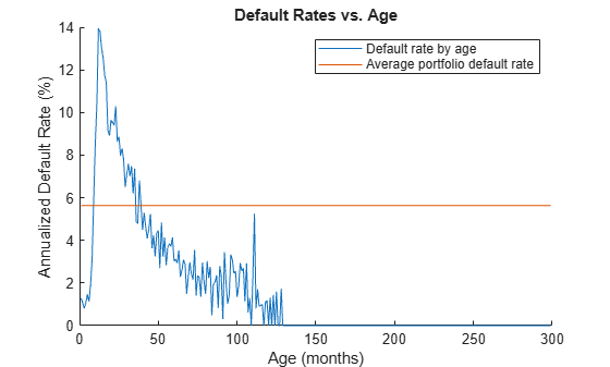
The figure shows that the annualized default rate for loans in the mortgageData portfolio starts low, spikes around 12 months, and begins to level out after 35 months when it intersects the average default rate line for a second time.
A seasoned portfolio contains loans with a mix of low, average, and high default risks. Create a vector that contains the indices of the rows in mortgageData that correspond to observations five years after the earliest origination dates for the loans.
seasonedIdx = year(mortgageData.ObservationDate) > 2004;
Default rates for mortgages typically rise when the unemployment rate rises. Plot the default rate together with the unemployment rate.
g = groupsummary(mortgageData,"ObservationDate","mean",["Default","UnemploymentRate_Lag0"]);

unemploymentRate = g.mean_UnemploymentRate_Lag0;
defaultRate = 100*(1-(1-g.mean_Default).^12);

figure;

yyaxis left
plot(g.ObservationDate,unemploymentRate)
ylabel("Unemployment Rate (%)")
xlabel("Date")

yyaxis right;
plot(g.ObservationDate,defaultRate)
ylabel("Annualized Default Rate (%)")

title("Unemployment Rates and Default Rates")
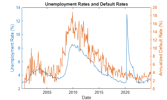
The figure shows that, in the first five years, the default rate for the portfolio is very low. This result is consistent with the results in the Default Rate vs. Age figure. As the portfolio becomes more seasoned, the default rate trend follows the unemployment rate trend. The unemployment rate reaches a local maximum after the 2008 financial crisis then trends downward until it spikes sharply in 2020 during the Covid-19 pandemic.
Partition Data
During the pandemic, the default rate did not rise with the unemployment rate due to pandemic financial assistance. Create a vector of indices for the rows in mortgageData corresponding to observations before the pandemic unemployment spike.
preCovidIdx = year(mortgageData.ObservationDate) < 2020;
Define an in-sample data set for years 2005 to 2019 by using the cvpartition function.
sampleIdx = seasonedIdx & preCovidIdx;
rng(0,"twister")
cv = cvpartition(mortgageData{sampleIdx,"ObservationDate"},Holdout=0.3);
Partition the in-sample data into a training set and test set.
trainingIdx = [false(sum(~seasonedIdx),1);training(cv);false(sum(~preCovidIdx),1)];
testIdx = [false(sum(~seasonedIdx),1);test(cv);false(sum(~preCovidIdx),1)];
Add a variable to the mortgage payment data indicating whether an observation is in the unseasoned, training, test, or out-of-sample set. The unseasoned data set contains data with observation years of 2004 and earlier. The out-of-sample data contains the data with observation years of 2020 and later.
mortgageData{:,"Sample"} = categorical(nan);
mortgageData{~seasonedIdx,"Sample"} = categorical("Unseasoned");
mortgageData{trainingIdx,"Sample"} = categorical("Train");
mortgageData{testIdx,"Sample"} = categorical("Test");
mortgageData{~preCovidIdx,"Sample"} = categorical("Out of Sample");
Bin Data
The annualized default and payoff rates are assumed to, respectively, decrease and increase as the origination credit scores increase. Use the discretize function to bin the training sample's OriginationCreditScore data such that the assumptions hold. You can use the Binning Explorer app to find the bins. Plot the default and payoff rates against the binned credit score data.
mortgageData.BinnedOriginationCreditScore = discretize(mortgageData.OriginationCreditScore,[300,600,700,750,800,850],"categorical");
g = groupsummary(mortgageData(trainingIdx,:),"BinnedOriginationCreditScore","mean",["Default","Payoff"]);

tiledlayout("horizontal");
nexttile
bar(g.BinnedOriginationCreditScore,100*(1-(1-g.mean_Default).^12))
title("Credit Score vs. Default Rate")
xlabel("Credit Score")
ylabel("Default Rate (%)")
nexttile
bar(g.BinnedOriginationCreditScore,100*(1-(1-g.mean_Payoff).^12))
title("Credit Score vs. Payoff Rate")
xlabel("Credit Score")
ylabel("Payoff Rate (%)")
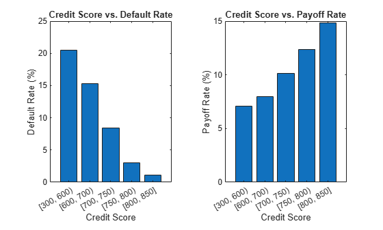
The figures show that the chosen bins result in a default rate that decreases and a payoff rate that increases as the credit score increases.
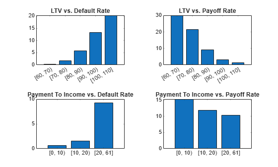
The annualized default rate is assumed to increase with the origination LTV score and origination payment-to-income ratio and the annualized payoff rate is assumed to decrease with those same variables. Bin the OriginationLTV and OriginationPaymentToIncome variables such that the assumptions hold. Plot default and payment rates against the binned LTV and payment-to-income ratio data.
mortgageData.BinnedOriginationLTV = discretize(mortgageData.OriginationLTV,60:10:110,"categorical");
g1 = groupsummary(mortgageData(trainingIdx,:),"BinnedOriginationLTV","mean",["Default","Payoff"]);

mortgageData.BinnedOriginationPaymentToIncome = discretize(mortgageData.OriginationPaymentToIncome,[0,10,20,61],"categorical");
g2 = groupsummary(mortgageData(trainingIdx,:),"BinnedOriginationPaymentToIncome","mean",["Default","Payoff"]);

tiledlayout(2,2)
nexttile
bar(g1.BinnedOriginationLTV,100*(1-(1-g1.mean_Default).^12))
title("LTV vs. Default Rate")
nexttile
bar(g1.BinnedOriginationLTV,100*(1-(1-g1.mean_Payoff).^12))
title("LTV vs. Payoff Rate")
nexttile
bar(g2.BinnedOriginationPaymentToIncome,100*(1-(1-g2.mean_Default).^12))
title("Payment To Income vs. Default Rate")
nexttile
bar(g2.BinnedOriginationPaymentToIncome,100*(1-(1-g2.mean_Payoff).^12))
title("Payment To Income vs. Payoff Rate")
The Age variable is expected to have a nonmonotonic relationship with the default rate. In the Default Rates vs. Age figure, the default rate is low in the first few months after origination and peaks around one year. After the default rate peaks, it trends downward over the remaining lifetime of the loan. Borrowers who do not default in the initial seasoning period are more likely to continue making payments. Bin Age to capture these dynamics and calculate the group counts, mean defaults, and mean payoffs for each bin.
mortgageData.BinnedAge = discretize(mortgageData.Age,[0,7,13:12:49,85,360],"categorical");
g = groupsummary(mortgageData(trainingIdx,:),"BinnedAge","mean",["Default","Payoff"])
g=7×4 table
    BinnedAge    GroupCount    mean_Default    mean_Payoff
    _________    __________    ____________    ___________

    [0, 7)            77406     0.0014986       0.0022996
    [7, 13)           73566     0.0082511       0.0023924
    [13, 25)     1.2469e+05      0.011316       0.0057905
    [25, 37)          96570     0.0082324        0.008833
    [37, 49)          73608     0.0052576        0.011317
    [49, 85)     1.2034e+05     0.0037644        0.016745
    [85, 360]         38807     0.0027057        0.024712
tiledlayout("horizontal")
nexttile
bar(g.BinnedAge,100*(1-(1-g.mean_Default).^12))
title("Age vs. Default Rate")
nexttile
bar(g.BinnedAge,100*(1-(1-g.mean_Payoff).^12))
title("Age vs. Payoff Rate")
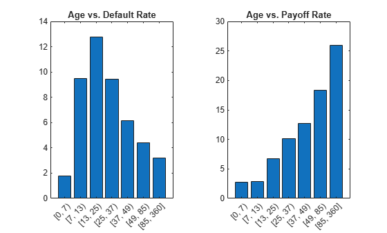
The plots show that, after seven years, the payoff rate increases as the portfolio age increases. This trend occurs because the loan balance decreases as the portfolio ages, making it easier for borrowers to pay off their loan. The trend also reflects the tendency of borrowers to change residences in the seven-to-ten year period.
Fit Multinomial Regression Model
Fit a multinomial regression model to the data in trainingSample. Use a response that indicates whether a scheduled payment corresponds to a default, payoff, or neither.
Select the macroeconomic variable predictors to use in the model. Ideal variables have good prediction power for both the probability of default and the probability of payoff. Exclude the date from the predictor candidates because it is not a macroeconomic variable.
macroVariables = string(macroEconData.Properties.VariableNames);
macroVariables = macroVariables(macroVariables ~= "Date");
Investigate which macroeconomic variables have good prediction power for the probability of default using the screenpredictors function. Sort the calculated values for the predictor screening metrics by using the AUROC values.
screenPredictorsDefault = mortgageData(trainingIdx,[macroVariables,"Default"]);
screenPredictorsDefault = screenpredictors(screenPredictorsDefault,"ResponseVar","Default");
screenPredictorsDefault = sortrows(screenPredictorsDefault,"AUROC","descend");
head(screenPredictorsDefault,23);
                                 InfoValue    AccuracyRatio     AUROC     Entropy       Gini      Chi2PValue     PercentMissing
                                 _________    _____________    _______    ________    ________    ___________    ______________

    UnemploymentRate_Lag0         0.27184        0.28785       0.64392    0.054608    0.012701    1.9668e-234          0
    UnemploymentRate_Lag3         0.25046        0.27661        0.6383    0.054713    0.012703    8.8767e-212          0
    HousingPriceIndex_Lag0        0.23869        0.26181       0.63091    0.054767    0.012704    5.0445e-201          0
    UnemploymentRate_Lag6         0.23015        0.25741       0.62871    0.054811    0.012705    8.6773e-190          0
    HousingPriceIndex_Lag3        0.24019        0.25361        0.6268    0.054765    0.012704    1.7446e-200          0
    HousingPriceIndex_Lag6        0.22555        0.24978       0.62489    0.054835    0.012705    1.7596e-185          0
    EquityIndex_Lag0               0.1978        0.23624       0.61812    0.054964    0.012708    1.8062e-161          0
    HousingPriceIndex_Lag9        0.19211        0.23432       0.61716    0.055001    0.012709    1.7305e-147          0
    UnemploymentRate_Lag9         0.19192        0.23206       0.61603    0.054984    0.012708    9.2202e-158          0
    EquityIndex_Lag3              0.19336        0.23048       0.61524    0.054985    0.012708    1.1654e-156          0
    EquityIndex_Lag6              0.17817        0.21747       0.60873    0.055063     0.01271    7.3755e-138          0
    HousingPriceIndex_Lag12       0.17639        0.21283       0.60641    0.055088    0.012711      6.55e-125          0
    EquityIndex_Lag9              0.17805        0.21056       0.60528    0.055071    0.012711    4.5916e-133          0
    UnemploymentRate_Lag12        0.17999        0.20457       0.60229    0.055043    0.012709    6.0328e-145          0
    EquityIndex_Lag12             0.17891        0.20386       0.60193    0.055073    0.012711    1.1707e-130          0
    HousingPriceIndex_Rel12       0.15534        0.15147       0.57574    0.055153    0.012712    2.4639e-122          0
    ConsumerPriceIndex_Lag0       0.28668        0.14642       0.57321    0.054549      0.0127     4.224e-248          0
    ConsumerPriceIndex_Lag3       0.28034        0.14306       0.57153    0.054578      0.0127    5.9671e-241          0
    ConsumerPriceIndex_Lag12      0.28668        0.14077       0.57038    0.054549      0.0127     4.224e-248          0
    ConsumerPriceIndex_Lag6       0.28144        0.13913       0.56956    0.054575      0.0127    5.9176e-241          0
    ConsumerPriceIndex_Lag9       0.28337        0.13833       0.56917    0.054562      0.0127    3.4389e-245          0
    HousingPriceIndex_Rel9        0.12774        0.12922       0.56461     0.05527    0.012713    7.0509e-106          0
    AverageMortgageRate_Rel12     0.11533        0.12446       0.56223    0.055348    0.012716     8.8505e-82          0
By AUROC, the first, third, and twenty-third strongest predictors for Default are UnemploymentRate_Lag0, HousingPriceIndex_Lag0, and AverageMortgageRate_Rel12.
Investigate which macroeconomic variables have good prediction power for the probability of payoff.
screenPredictorsPayoff = mortgageData(trainingIdx,[macroVariables,"Payoff"]);
screenPredictorsPayoff = screenpredictors(screenPredictorsPayoff,"ResponseVar","Payoff");
screenPredictorsPayoff = sortrows(screenPredictorsPayoff,"AUROC","descend");
head(screenPredictorsPayoff);
                                   InfoValue    AccuracyRatio     AUROC     Entropy       Gini      Chi2PValue     PercentMissing
                                   _________    _____________    _______    ________    ________    ___________    ______________

    AverageMortgageRate_Rel12       0.17154        0.21199       0.60599    0.076201    0.018753    4.8071e-190          0
    HousingPriceIndex_Lag0          0.24485        0.19219        0.5961    0.075725    0.018741    7.4746e-277          0
    UnemploymentRate_Lag0           0.22658         0.1893       0.59465    0.075814    0.018741    2.1465e-272          0
    HousingPriceIndex_Lag3          0.23175        0.18915       0.59457    0.075811    0.018742    1.3719e-263          0
    UnemploymentRate_Lag3           0.20609        0.18033       0.59016    0.075942    0.018744    2.0468e-250          0
    HousingPriceIndex_Lag6          0.18978        0.18029       0.59014    0.076086     0.01875    4.2992e-212          0
    BenchmarkInterestRate_Rel12     0.12805        0.17655       0.58827    0.076484    0.018761    1.4394e-139          0
    AverageMortgageRate_Rel9        0.12676        0.17464       0.58732    0.076486     0.01876    1.2363e-141          0
The first, second, and third strongest predictors for Payoff are AverageMortgageRate_Rel12, HousingPriceIndex_Lag0, and UnemploymentRate_Lag0. This result indicates that these variables have good predictive power for both the probability of default and the probability of payoff.
Investigate the correlation between AverageMortgageRate_Rel12, HousingPriceIndex_Lag0, and UnemploymentRate_Lag0 over the time period of interest.
idx = macroEconData.Date >= min(mortgageData{trainingIdx,"ObservationDate"}) & macroEconData.Date <= max(mortgageData{trainingIdx,"ObservationDate"});
corr(macroEconData{idx, ["AverageMortgageRate_Rel12","HousingPriceIndex_Lag0","UnemploymentRate_Lag0"]})
ans = 3×3
1.0000 0.2530 -0.3430
0.2530 1.0000 -0.7329
-0.3430 -0.7329 1.0000
The correlation between HousingPriceIndex_Lag0 and UnemploymentRate_Lag0 is relatively high. Use AverageMortgageRate_Rel12 and UnemploymentRate_Lag0 as macroeconomic predictors for the model.
Add a multinomial response variable to the trainingSample data set.
mortgageData{:,"MultinomialResponse"} = categorical(nan);
idx = mortgageData.Default == 1;
mortgageData{idx, "MultinomialResponse"} = categorical(repmat("Default",sum(idx),1));
idx = mortgageData.Payoff == 1;
mortgageData{idx, "MultinomialResponse"} = categorical(repmat("Payoff",sum(idx),1));
idx = mortgageData.Default == 0 & mortgageData.Payoff == 0;
mortgageData{idx, "MultinomialResponse"} = categorical(repmat("Survival",sum(idx),1));
MultinomialResponse is a categorical table variable with categories "Default", "Payoff", and "Survival". These categories indicate whether an observation corresponds to a mortgage default, payoff, or neither.
Fit a multinomial regression model to the data in trainingSample. Use MultinomialResponse as the response variable, and the mortgage payment data together with AverageMortgageRate_Rel12 and UnemploymentRate_Lag0 as the model predictors.
predsResponse = mortgageData(trainingIdx,["BinnedAge","BinnedOriginationCreditScore","BinnedOriginationLTV", ...
    "BinnedOriginationPaymentToIncome","AverageMortgageRate_Rel12","UnemploymentRate_Lag0","MultinomialResponse"]);
model = fitmnr(predsResponse,"MultinomialResponse");
disp(model.Coefficients)
                                                          Value         SE         tStat       pValue
                                                         ________    _________    _______    ___________

    (Intercept_Default)                                   -12.287      0.73792     -16.65     3.0116e-62
    BinnedAge_[7, 13)_Default                              1.7765      0.10178     17.454     3.2338e-68
    BinnedAge_[13, 25)_Default                             2.2284      0.09703     22.966    1.0272e-116
    BinnedAge_[25, 37)_Default                             1.9773     0.099927     19.787     3.8303e-87
    BinnedAge_[37, 49)_Default                             1.4857      0.10648     13.953     2.9971e-44
    BinnedAge_[49, 85)_Default                            0.99327      0.10477     9.4804     2.5338e-21
    BinnedAge_[85, 360]_Default                           0.37952      0.13599     2.7909      0.0052569
    BinnedOriginationCreditScore_[600, 700)_Default      -0.13605     0.063187    -2.1531       0.031313
    BinnedOriginationCreditScore_[700, 750)_Default      -0.76253     0.058329    -13.073     4.6965e-39
    BinnedOriginationCreditScore_[750, 800)_Default       -1.7767     0.068222    -26.043    1.6189e-149
    BinnedOriginationCreditScore_[800, 850]_Default       -2.6654      0.25625    -10.401      2.444e-25
    BinnedOriginationLTV_[70, 80)_Default                  1.3804      0.58228     2.3707       0.017753
    BinnedOriginationLTV_[80, 90)_Default                  2.6163      0.57842     4.5231     6.0952e-06
    BinnedOriginationLTV_[90, 100)_Default                 3.4081      0.57834     5.8929     3.7939e-09
    BinnedOriginationLTV_[100, 110]_Default                3.7078      0.57951     6.3982     1.5723e-10
    BinnedOriginationPaymentToIncome_[10, 20)_Default     0.75328       0.4538     1.6599        0.09693
    BinnedOriginationPaymentToIncome_[20, 61]_Default       2.342      0.44804     5.2271     1.7218e-07
    AverageMortgageRate_Rel12_Default                    -0.16453      0.14501    -1.1346        0.25652
    UnemploymentRate_Lag0_Default                         0.30793    0.0091544     33.638    4.7313e-248
    (Intercept_Payoff)                                    -5.4366       0.1569     -34.65    4.4911e-263
    BinnedAge_[7, 13)_Payoff                             0.077119      0.10662    0.72328        0.46951
    BinnedAge_[13, 25)_Payoff                              1.0065     0.084059     11.974     4.8753e-33
    BinnedAge_[25, 37)_Payoff                               1.493      0.08292     18.006     1.7583e-72
    BinnedAge_[37, 49)_Payoff                              1.8408     0.083233     22.116    2.2097e-108
    BinnedAge_[49, 85)_Payoff                              2.4667     0.079162     31.161    3.6297e-213
    BinnedAge_[85, 360]_Payoff                             3.3123     0.084098     39.386              0
    BinnedOriginationCreditScore_[600, 700)_Payoff       0.030022      0.10457     0.2871        0.77404
    BinnedOriginationCreditScore_[700, 750)_Payoff       0.046062     0.095627    0.48168        0.63003
    BinnedOriginationCreditScore_[750, 800)_Payoff        0.10047     0.095523     1.0518        0.29291
    BinnedOriginationCreditScore_[800, 850]_Payoff         0.1385       0.1148     1.2064        0.22766
    BinnedOriginationLTV_[70, 80)_Payoff                 -0.64348     0.061842    -10.405     2.3455e-25
    BinnedOriginationLTV_[80, 90)_Payoff                  -2.0501     0.064002    -32.033    3.8279e-225
    BinnedOriginationLTV_[90, 100)_Payoff                 -3.3789     0.080518    -41.964              0
    BinnedOriginationLTV_[100, 110]_Payoff                -4.1444      0.18765    -22.086    4.3475e-108
    BinnedOriginationPaymentToIncome_[10, 20)_Payoff     -0.21574     0.091009    -2.3706       0.017761
    BinnedOriginationPaymentToIncome_[20, 61]_Payoff     -0.24636     0.088715     -2.777       0.005487
    AverageMortgageRate_Rel12_Payoff                       -1.993      0.11877    -16.781     3.3858e-63
    UnemploymentRate_Lag0_Payoff                          0.17065    0.0072024     23.693    4.2096e-124
A large p-value for a coefficient indicates that its corresponding term does not have a statistically significant effect on the response. The results in the output indicate that AverageMortgageRate_Rel12 does not have a significant effect on the default rate. The coefficient signs for the mortgage payment variables are consistent with industry-assumed relationships.
Predict default and payoff rates
Use the predict function to predict whether the observations in fullSample correspond to a mortgage default, payoff, or neither. Create two new table variables to store the results.
[~, probs] = predict(model,mortgageData);
mortgageData{:,["PredictedDefault", "PredictedPayoff"]} = probs(:,[1,2]);
Plot the annualized default and payoff rates for the training, test, and out-of-sample data. For each payment date, calculate the means for the Default, Payoff, PredictedDefault, and PredictedPayoff variables.
g = groupsummary(mortgageData,["ObservationDate", "Sample"],"mean",["Default","Payoff","PredictedDefault","PredictedPayoff"]);

idxTrain = g.Sample == "Train";
idxTest = g.Sample == "Test";
idxOOS = g.Sample == "Out of Sample";
trainDates = g.ObservationDate(idxTrain);
trainActualDefault = 100*(1-(1-g(idxTrain,:).("mean_Default")).^12);
trainActualPayoff = 100*(1-(1-g(idxTrain,:).("mean_Payoff")).^12);
trainPredictedDefault = 100*(1-(1-g(idxTrain,:).("mean_PredictedDefault")).^12);
trainPredictedPayoff = 100*(1-(1-g(idxTrain,:).("mean_PredictedPayoff")).^12);

testDates = g.ObservationDate(idxTest);
testActualDefault = 100*(1-(1-g(idxTest,:).("mean_Default")).^12);
testActualPayoff = 100*(1-(1-g(idxTest,:).("mean_Payoff")).^12);
testPredictedDefault = 100*(1-(1-g(idxTest,:).("mean_PredictedDefault")).^12);
testPredictedPayoff = 100*(1-(1-g(idxTest,:).("mean_PredictedPayoff")).^12);

oosDates = g.ObservationDate(idxOOS);
oosActualDefault = 100*(1-(1-g(idxOOS,:).("mean_Default")).^12);
oosActualPayoff = 100*(1-(1-g(idxOOS,:).("mean_Payoff")).^12);
oosPredictedDefault = 100*(1-(1-g(idxOOS,:).("mean_PredictedDefault")).^12);
oosPredictedPayoff = 100*(1-(1-g(idxOOS,:).("mean_PredictedPayoff")).^12);

tiledlayout(3,2)

nexttile
plot(trainDates,[trainActualDefault,trainPredictedDefault])
title("Default")
ylabel("Train",FontWeight="bold")
legend("Actual","Predicted")

nexttile
plot(trainDates,[trainActualPayoff,trainPredictedPayoff])
title("Payoff")

nexttile
plot(testDates,[testActualDefault,testPredictedDefault])
ylabel("Test",FontWeight="bold")

nexttile
plot(testDates,[testActualPayoff,testPredictedPayoff])
nexttile
plot(oosDates,[oosActualDefault,oosPredictedDefault])
ylabel("Out of Sample",FontWeight="bold")

nexttile
plot(oosDates,[oosActualPayoff,oosPredictedPayoff])
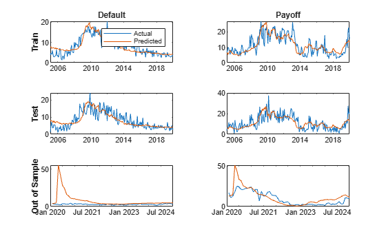
In the training and test data, each predicted outcome curve follows the same trends as its corresponding actual outcome curve. In the out-of-sample data, the predicted default undergoes a large spike and quick recovery corresponding to unemployment dynamics during the Covid-19 pandemic. In the post Covid-19 period, defaults tend to be lower than modeled. The model captures but overshoots the pandemic payoff episode in the out-of-sample data. Although it captures the dip immediately after the payoff period, it predicts higher payoff rates.
See Also
mnrfit | MultinomialRegression | Binning Explorer | fitLifetimePDModel