Reorder RF Components to Optimize X-Band RF Receiver Sensitivity
R2026bThis example shows how to optimize the sensitivity of an X-band (9.4 GHz) RF receiver by reordering components in the signal chain. Using the rfbudget object, you compare three configurations, verify specification compliance, and validate the winning design with harmonic balance analysis.
In receiver design, the order in which components are arranged has a dramatic impact on overall sensitivity and dynamic range. This is a direct consequence of Friis' cascade noise figure formula:
NF_sys = NF1 + (NF2-1)/G1 + (NF3-1)/(G1*G2) + ...
The formula shows that the noise figure of the first stage dominates the system NF. Each subsequent stage contribution is divided by the cumulative gain of all preceding stages. This means:
A low-noise amplifier (LNA) first minimizes system NF because its high gain suppresses noise from later stages.
A lossy element first (filter or mixer) degrades sensitivity because its noise contribution is not attenuated by any preceding gain.
Define X-Band Receiver Specifications
The specifications below are representative of an X-band RF receiver operating at 9.4 GHz. The intermediate frequency (IF) is chosen at 1.4 GHz to provide adequate image rejection and allow practical IF filter design.
spec.Frequency    = 9.4e9;     % Hz  - X-band center
spec.IF           = 1.4e9;     % Hz  - Intermediate frequency
spec.Bandwidth    = 10e6;      % Hz  - Channel bandwidth
spec.Sensitivity  = -90;       % dBm - Minimum detectable signal
spec.RequiredSNR  = 10;        % dB  - Required output SNR
spec.MaxNF        = 4;         % dB  - Noise figure limit
spec.MinGain      = 25;        % dB  - Minimum system gain
spec.MinOIP3      = 10;        % dBm - Linearity target

% Derived local oscillator (LO) frequency (low-side injection)
spec.LOFrequency = spec.Frequency - spec.IF;  % 8.0 GHz
Select X-Band RF Components
At 9.4 GHz, LNA noise figures are typically 1.5-2.5 dB (vs. <1 dB at 2 GHz), filter insertion losses are higher, and mixers have greater conversion loss. Each component is defined once and then cloned for reuse across configurations.
inputFreq = spec.Frequency;
inputPower = -50;                % dBm - nominal test power
bandwidth = spec.Bandwidth;
loFreq = spec.LOFrequency;
Low-Noise Amplifier (LNA) - Sets the system noise figure. At X-band, GaAs pHEMT LNAs typically achieve 1.8-2.2 dB NF with 12-18 dB gain. Higher gain here is critical because it suppresses the noise of all following stages.
lna = amplifier(Name="LNA", Gain=18, NF=2.0, OIP3=28);
RF Bandpass Filter (BPF) - A waveguide or cavity bandpass filter centered at 9.4 GHz. It rejects out-of-band interference and image frequency signals. X-band filters have higher insertion loss (3-4 dB) than their lower-frequency counterparts.
bpf = amplifier(Name="BPF", Gain=-3.5, NF=3.5, OIP3=Inf);
Mixer (Down Converter) - Translates the 9.4 GHz RF signal to 1.4 GHz IF using an 8.0 GHz LO. Double-balanced diode mixers at X-band typically have 7-8 dB conversion loss and moderate linearity.
mixer = modulator(Name="Mixer", Gain=-7.5, NF=7, OIP3=13, OIP2=28, ...
    LO=loFreq, ConverterType="Down");
IF Bandpass Filter (IF BPF) - A ceramic or surface acoustic wave (SAW) filter centered at the 1.4 GHz IF frequency. It rejects mixer spurs, LO leakage, and image products that fall outside the desired IF band.
ifBpf = amplifier(Name="IF_BPF", Gain=-1.5, NF=1.5, OIP3=Inf);
IF Amplifier - Provides gain at the 1.4 GHz intermediate frequency. IF amplifiers have better NF than X-band components because they operate at a lower frequency. The gain is chosen to meet the system gain requirement.
ifAmp = amplifier(Name="IFAmp", Gain=28, NF=3.5, OIP3=22);
Compare Three Component Orderings
To understand the effect of component ordering, build three candidate configurations using the same components in different orders. Each arrangement represents a distinct design philosophy:
Configuration A (LNA First) - Placing the LNA first minimizes the system noise figure.
Configuration B (Filter First) - Places the bandpass filter before the LNA. This protects the LNA from strong out-of-band interference but sacrifices 3.5 dB of noise performance.
Configuration C (Mixer First) - An intentionally poor arrangement where the mixer is placed at the front of the chain. This results in the worst noise figure.
cloneSet = @() struct( ...
    'lna',  clone(lna),  'bpf', clone(bpf), ...
    'mixer',clone(mixer),'ifBpf',clone(ifBpf),'ifAmp',clone(ifAmp));

% Configuration A - LNA First (Classic Low-Noise Design)
cA = cloneSet();
configA = rfbudget([cA.lna, cA.bpf, cA.mixer, cA.ifBpf, cA.ifAmp], ...
    inputFreq, inputPower, bandwidth);

% Configuration B - Filter First (Interferer Protection)
cB = cloneSet();
configB = rfbudget([cB.bpf, cB.lna, cB.mixer, cB.ifBpf, cB.ifAmp], ...
    inputFreq, inputPower, bandwidth);

% Configuration C - Mixer First (Poor Design)
cC = cloneSet();
configC = rfbudget([cC.mixer, cC.lna, cC.bpf, cC.ifBpf, cC.ifAmp], ...
    inputFreq, inputPower, bandwidth);
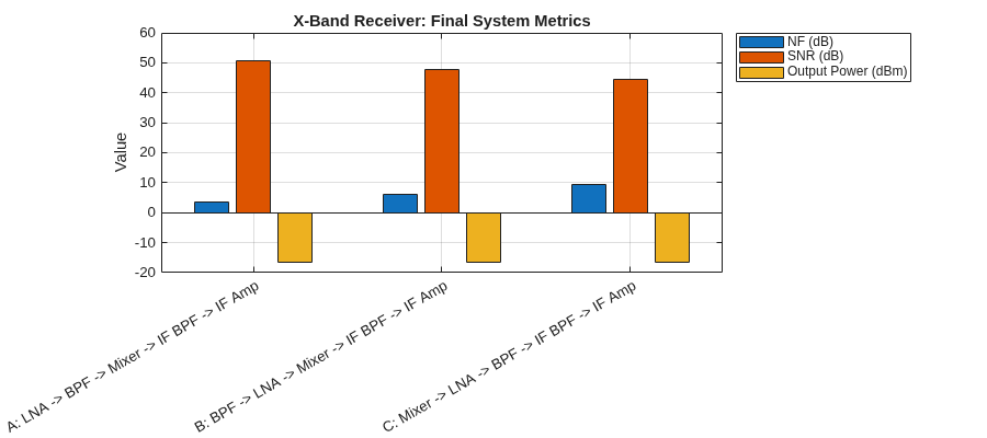
Display the budget results for all three configurations side by side. The output shows each configuration's total gain, noise figure, SNR, output power, and OIP3. Configuration A (LNA first) achieves the lowest NF and highest SNR, confirming the importance of placing a high-gain, low-noise stage first in the chain.
configs = {configA, configB, configC};
configLabels = [ ...
    "A: LNA -> BPF -> Mixer -> IF BPF -> IF Amp", ...
    "B: BPF -> LNA -> Mixer -> IF BPF -> IF Amp", ...
    "C: Mixer -> LNA -> BPF -> IF BPF -> IF Amp"];

txt = [ ...
    "=================================================================" ; ...
    "  X-BAND RF BUDGET - EFFECT OF COMPONENT ORDERING" ; ...
    sprintf("  Input: %.1f GHz | %.0f dBm | %.0f MHz BW", ...
    inputFreq/1e9, inputPower, bandwidth/1e6) ; ...
    "=================================================================" ];
for k = 1:3
    c = configs{k};
    oip3 = c.OIP3(end);
    if isinf(oip3), oip3Str = "   Inf"; else, oip3Str = sprintf("%6.1f", oip3); end
    txt = [txt ; "" ; ...  %#ok<AGROW>
        sprintf("  Config %s", configLabels(k)) ; ...
        sprintf("    Total Gain  : %6.1f dB", c.TransducerGain(end)) ; ...
        sprintf("    Noise Figure: %6.2f dB", c.NF(end)) ; ...
        sprintf("    SNR         : %6.2f dB", c.SNR(end)) ; ...
        sprintf("    Output Power: %6.1f dBm", c.OutputPower(end)) ; ...
        sprintf("    OIP3        : %s dBm", oip3Str) ];
end
disp(strjoin(txt, newline));
=================================================================
  X-BAND RF BUDGET - EFFECT OF COMPONENT ORDERING
  Input: 9.4 GHz | -50 dBm | 10 MHz BW
=================================================================

  Config A: LNA -> BPF -> Mixer -> IF BPF -> IF Amp
    Total Gain  :   33.5 dB
    Noise Figure:   3.38 dB
    SNR         :  50.59 dB
    Output Power:  -16.5 dBm
    OIP3        :   21.9 dBm

  Config B: BPF -> LNA -> Mixer -> IF BPF -> IF Amp
    Total Gain  :   33.5 dB
    Noise Figure:   6.15 dB
    SNR         :  47.82 dB
    Output Power:  -16.5 dBm
    OIP3        :   21.9 dBm

  Config C: Mixer -> LNA -> BPF -> IF BPF -> IF Amp
    Total Gain  :   33.5 dB
    Noise Figure:   9.47 dB
    SNR         :  44.51 dB
    Output Power:  -16.5 dBm
    OIP3        :   22.0 dBm
Plot a bar chart comparing the final NF, SNR, and output power across all three configurations.
figure('Name','X-Band Final Metrics','Position',[200 150 900 400]);
metricNames = ["NF (dB)", "SNR (dB)", "Output Power (dBm)"];
metricData = zeros(3,3);
for k = 1:3
    metricData(k,:) = [configs{k}.NF(end), configs{k}.SNR(end), ...
        configs{k}.OutputPower(end)];
end
bar(metricData);
xticklabels(configLabels);
ylabel('Value'); legend(metricNames, Location="bestoutside");
title('X-Band Receiver: Final System Metrics');
grid on;
Visualize Stage-by-Stage Performance
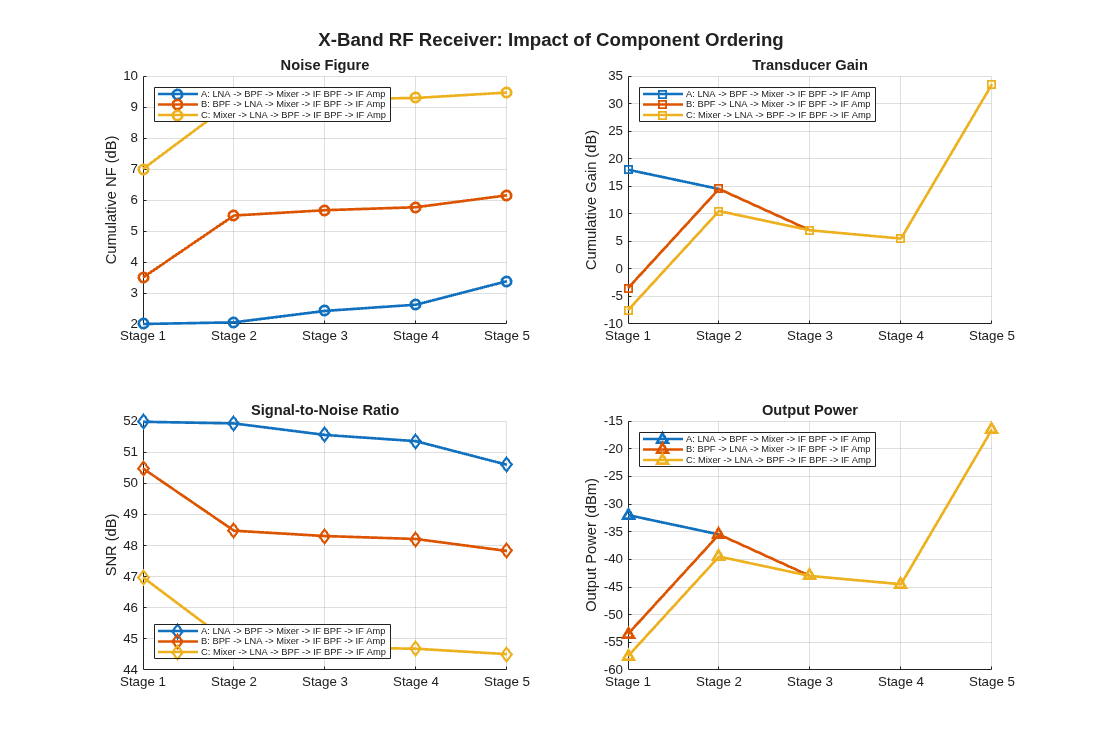
Visualize the performance of the receiver to analyze how noise figure, gain, SNR, and output power evolve as the signal passes through each stage. The curves reveal the impact of component ordering at each point in the receive chain.
stageLabels = ["Stage 1", "Stage 2", "Stage 3", "Stage 4", "Stage 5"];
nStages = 5;
colors = lines(3);

figure('Name','X-Band Component Ordering Comparison', ...
    'Position',[100 80 1100 750]);

subplot(2,2,1);
hold on;
for k = 1:3
    plot(1:nStages, configs{k}.NF, '-o', 'LineWidth', 2, ...
        'MarkerSize', 7, 'Color', colors(k,:));
end
hold off;
xticks(1:nStages); xticklabels(stageLabels);
ylabel('Cumulative NF (dB)'); title('Noise Figure');
legend(configLabels, Location="northwest", FontSize=7);
grid on;

subplot(2,2,2);
hold on;
for k = 1:3
    plot(1:nStages, configs{k}.TransducerGain, '-s', 'LineWidth', 2, ...
        'MarkerSize', 7, 'Color', colors(k,:));
end
hold off;
xticks(1:nStages); xticklabels(stageLabels);
ylabel('Cumulative Gain (dB)'); title('Transducer Gain');
legend(configLabels, Location="northwest", FontSize=7);
grid on;

subplot(2,2,3);
hold on;
for k = 1:3
    plot(1:nStages, configs{k}.SNR, '-d', 'LineWidth', 2, ...
        'MarkerSize', 7, 'Color', colors(k,:));
end
hold off;
xticks(1:nStages); xticklabels(stageLabels);
ylabel('SNR (dB)'); title('Signal-to-Noise Ratio');
legend(configLabels, Location="southwest", FontSize=7);
grid on;

subplot(2,2,4);
hold on;
for k = 1:3
    plot(1:nStages, configs{k}.OutputPower, '-^', 'LineWidth', 2, ...
        'MarkerSize', 7, 'Color', colors(k,:));
end
hold off;
xticks(1:nStages); xticklabels(stageLabels);
ylabel('Output Power (dBm)'); title('Output Power');
legend(configLabels, Location="northwest", FontSize=7);
grid on;

sgtitle('X-Band RF Receiver: Impact of Component Ordering', ...
    'FontSize', 14, 'FontWeight', 'bold');
Verify Specification Compliance
A configuration passes only if it satisfies all receiver requirements simultaneously. At X-band, the noise figure specification is particularly challenging because components inherently have higher NF than at lower frequencies. This makes component ordering even more critical.
totalChecks = 4;
for k = 1:3
    c = configs{k};
    gainOK(k) = c.TransducerGain(end) >= spec.MinGain;
    nfOK(k) = c.NF(end) <= spec.MaxNF;
    oip3Val = c.OIP3(end);
    if isinf(oip3Val), oip3Val = 999; end
    oip3OK(k) = oip3Val >= spec.MinOIP3;
end

% Recompute at sensitivity to check SNR
cSens = {cloneSet(), cloneSet(), cloneSet()};
orders = {[cSens{1}.lna, cSens{1}.bpf, cSens{1}.mixer, cSens{1}.ifBpf, cSens{1}.ifAmp], ...
    [cSens{2}.bpf, cSens{2}.lna, cSens{2}.mixer, cSens{2}.ifBpf, cSens{2}.ifAmp], ...
    [cSens{3}.mixer, cSens{3}.lna, cSens{3}.bpf, cSens{3}.ifBpf, cSens{3}.ifAmp]};
for k = 1:3
    bSens = rfbudget(orders{k}, inputFreq, spec.Sensitivity, bandwidth);
    snrAtSens(k) = bSens.SNR(end);
    snrOK(k) = snrAtSens(k) >= spec.RequiredSNR;
end
Build and display the compliance table. Each configuration is checked against the gain, NF, OIP3, and SNR requirements. A PASS/FAIL verdict is shown for each metric, and the overall result identifies which configuration meets all specifications simultaneously.
checkNames = [ ...
    "Gain >= " + spec.MinGain + " dB", ...
    "NF <= " + spec.MaxNF + " dB", ...
    "OIP3 >= " + spec.MinOIP3 + " dBm", ...
    "SNR >= " + spec.RequiredSNR + " dB @ " + spec.Sensitivity + " dBm"];
checkResults = [gainOK; nfOK; oip3OK; snrOK];

sep = repmat('-',1,35);
txt = [ ...
    "=================================================================" ; ...
    "  SPECIFICATION COMPLIANCE CHECK" ; ...
    "=================================================================" ; ...
    sprintf("  %-35s  %8s  %8s  %8s", "Requirement", "Config A", "Config B", "Config C") ; ...
    sprintf("  %-35s  %8s  %8s  %8s", sep, "--------", "--------", "--------") ];
for j = 1:totalChecks
    symbols = strings(1,3);
    for k = 1:3
        if checkResults(j,k), symbols(k) = "  PASS"; else, symbols(k) = "  FAIL"; end
    end
    txt = [txt ; sprintf("  %-35s  %8s  %8s  %8s", checkNames(j), symbols(1), symbols(2), symbols(3))]; %#ok<AGROW>
end
overallPass = gainOK & nfOK & oip3OK & snrOK;
verdict = strings(1,3);
for k = 1:3
    if overallPass(k), verdict(k) = "  PASS"; else, verdict(k) = "  FAIL"; end
end
txt = [txt ; ...
    sprintf("  %-35s  %8s  %8s  %8s", sep, "--------", "--------", "--------") ; ...
    sprintf("  %-35s  %8s  %8s  %8s", "OVERALL", verdict(1), verdict(2), verdict(3)) ; ...
    "=================================================================" ];
passingIdx = find(overallPass);
if ~isempty(passingIdx)
    txt = [txt ; sprintf("  >> Configuration %s meets all X-band receiver specifications.", ...
        char('A' + passingIdx(1) - 1))];
else
    txt = [txt ; "  >> No configuration meets all specifications."];
end
disp(strjoin(txt, newline));
=================================================================
  SPECIFICATION COMPLIANCE CHECK
=================================================================
  Requirement                          Config A  Config B  Config C
  -----------------------------------  --------  --------  --------
  Gain >= 25 dB                            PASS      PASS      PASS
  NF <= 4 dB                               PASS      FAIL      FAIL
  OIP3 >= 10 dBm                           PASS      PASS      PASS
  SNR >= 10 dB @ -90 dBm                   PASS      FAIL      FAIL
  -----------------------------------  --------  --------  --------
  OVERALL                                  PASS      FAIL      FAIL
=================================================================
  >> Configuration A meets all X-band receiver specifications.
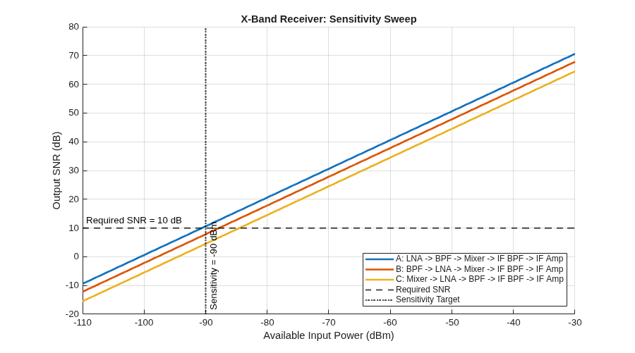
To determine the usable sensitivity range, sweep the available input power from -110 dBm (very weak signal) to -30 dBm (strong signal) and plot the output SNR for each configuration. This reveals which arrangement maintains adequate SNR at the lowest signal levels.
sweepPower = (-110:2:-30);
snrSweep = zeros(length(sweepPower), 3);
for p = 1:length(sweepPower)
    cS = {cloneSet(), cloneSet(), cloneSet()};
    ordersS = {[cS{1}.lna, cS{1}.bpf, cS{1}.mixer, cS{1}.ifBpf, cS{1}.ifAmp], ...
        [cS{2}.bpf, cS{2}.lna, cS{2}.mixer, cS{2}.ifBpf, cS{2}.ifAmp], ...
        [cS{3}.mixer, cS{3}.lna, cS{3}.bpf, cS{3}.ifBpf, cS{3}.ifAmp]};
    for k = 1:3
        bSweep = rfbudget(ordersS{k}, inputFreq, sweepPower(p), bandwidth);
        snrSweep(p,k) = bSweep.SNR(end);
    end
end

figure('Name','X-Band Sensitivity Sweep','Position',[250 100 900 500]);
colors = lines(3);
hold on;
for k = 1:3
    plot(sweepPower, snrSweep(:,k), '-', 'LineWidth', 2, 'Color', colors(k,:));
end
yline(spec.RequiredSNR, '--k', sprintf('Required SNR = %d dB', spec.RequiredSNR), ...
    'LineWidth', 1.5, 'LabelHorizontalAlignment', 'left', 'FontSize', 10);
xline(spec.Sensitivity, ':k', sprintf('Sensitivity = %d dBm', spec.Sensitivity), ...
    'LineWidth', 1.5, 'LabelVerticalAlignment', 'bottom', 'FontSize', 10);
hold off;
xlabel('Available Input Power (dBm)');
ylabel('Output SNR (dB)');
title('X-Band Receiver: Sensitivity Sweep');
legend([configLabels, "Required SNR", "Sensitivity Target"], ...
    Location="southeast");
grid on;
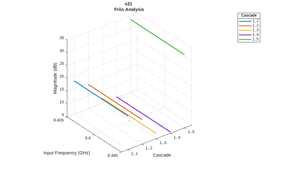
Display the full rfbudget table and RF chain plot for the best configuration. The table shows gain, NF, SNR, and IP3 at each stage, and the plot visualizes how these metrics accumulate through the chain.
if ~isempty(passingIdx)
    bestConfig = configs{passingIdx(1)};
    txt = [ ...
        "=================================================================" ; ...
        sprintf("  SELECTED DESIGN: Configuration %s", char('A' + passingIdx(1) - 1)) ; ...
        sprintf("  Order: %s", configLabels(passingIdx(1))) ; ...
        "=================================================================" ];
    disp(strjoin(txt, newline));
    disp(bestConfig);
    rfplot(bestConfig);
end
=================================================================
  SELECTED DESIGN: Configuration A
  Order: A: LNA -> BPF -> Mixer -> IF BPF -> IF Amp
=================================================================
  rfbudget with properties:

               Elements: [1x5 rf.internal.rfbudget.RFElement]
         InputFrequency: 9.4 GHz
    AvailableInputPower: -50 dBm
        SignalBandwidth:  10 MHz
                 Solver: Friis
             AutoUpdate: true

   Analysis Results
        OutputFrequency: (GHz) [  9.4    9.4    1.4    1.4     1.4]
            OutputPower: (dBm) [  -32  -35.5    -43  -44.5   -16.5]
         TransducerGain: (dB)  [   18   14.5      7    5.5    33.5]
                     NF: (dB)  [    2  2.053  2.423  2.623   3.381]
                   IIP3: (dBm) [   10     10  4.545  4.545  -11.61]
                   OIP3: (dBm) [   28   24.5  11.54  10.04   21.89]
                    SNR: (dB)  [51.98  51.92  51.55  51.35   50.59]
Validate Design with Harmonic Balance Analysis
In receivers with a low IF or direct-conversion architecture, IP2 matters because:
Strong interferers at f1 and f2 create IM2 products at f1-f2, which can fall at the IF frequency (1.4 GHz in this design).
This self-generated interference raises the effective noise floor and degrades the ability to receive weak signals.
To quantify these effects, compare Friis and Harmonic Balance results side by side for the winning configuration.
friisResult = configA;
cHB = cloneSet();
hbResult = rfbudget([cHB.lna, cHB.bpf, cHB.mixer, cHB.ifBpf, cHB.ifAmp], ...
    inputFreq, inputPower, bandwidth, ...
    Solver="HarmonicBalance", WaitBar=false);
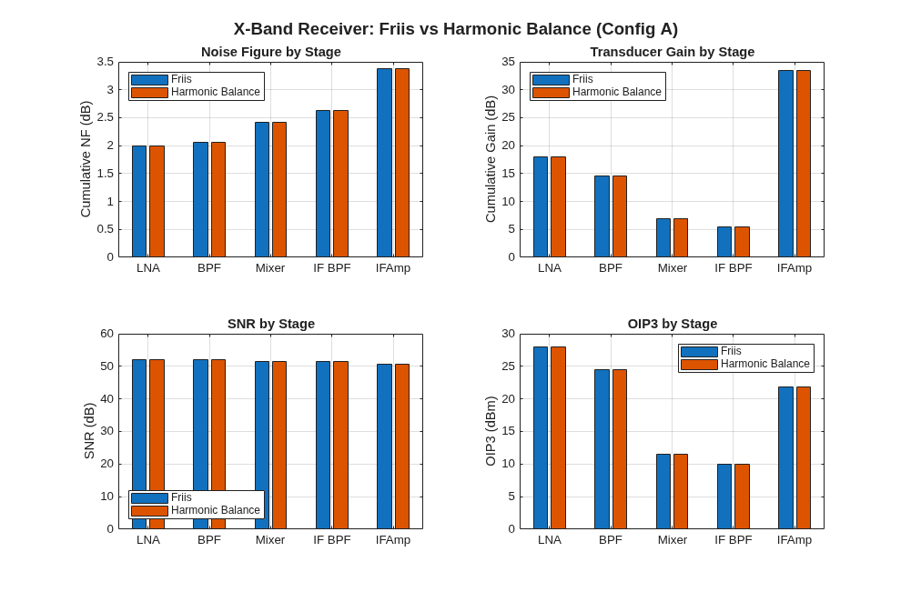
Build a comparison table showing Friis vs. Harmonic Balance results. The output reveals that gain, NF, and SNR are nearly identical between solvers at this nominal power level. The key difference is that the HB solver reports IIP2/OIP2 values, which the Friis solver cannot compute.
oip3F = friisResult.OIP3(end); oip3H = hbResult.OIP3(end);
if isinf(oip3F), oip3Fstr = "Inf"; else, oip3Fstr = sprintf("%.2f",oip3F); end
if isinf(oip3H), oip3Hstr = "Inf"; else, oip3Hstr = sprintf("%.2f",oip3H); end

iip2F = friisResult.IIP2; oip2F = friisResult.OIP2;
iip2H = hbResult.IIP2;    oip2H = hbResult.OIP2;
if isempty(iip2F), iip2Fstr = "N/A"; else, iip2Fstr = sprintf("%.2f",iip2F(end)); end
if isempty(oip2F), oip2Fstr = "N/A"; else, oip2Fstr = sprintf("%.2f",oip2F(end)); end
if isempty(iip2H), iip2Hstr = "N/A"; else, iip2Hstr = sprintf("%.2f",iip2H(end)); end
if isempty(oip2H), oip2Hstr = "N/A"; else, oip2Hstr = sprintf("%.2f",oip2H(end)); end

sep25 = repmat('-',1,25);
txt = [ ...
    "=================================================================" ; ...
    "  FRIIS vs HARMONIC BALANCE COMPARISON (Config A)" ; ...
    "=================================================================" ; ...
    sprintf("  %-25s  %12s  %12s", "Metric", "Friis", "Harmonic Bal") ; ...
    sprintf("  %-25s  %12s  %12s", sep25, "------------", "------------") ; ...
    sprintf("  %-25s  %12.2f  %12.2f", "Total Gain (dB)",    friisResult.TransducerGain(end), hbResult.TransducerGain(end)) ; ...
    sprintf("  %-25s  %12.2f  %12.2f", "Noise Figure (dB)",  friisResult.NF(end),             hbResult.NF(end)) ; ...
    sprintf("  %-25s  %12.2f  %12.2f", "SNR (dB)",           friisResult.SNR(end),             hbResult.SNR(end)) ; ...
    sprintf("  %-25s  %12.2f  %12.2f", "Output Power (dBm)", friisResult.OutputPower(end),     hbResult.OutputPower(end)) ; ...
    sprintf("  %-25s  %12s  %12s", "OIP3 (dBm)", oip3Fstr, oip3Hstr) ; ...
    sprintf("  %-25s  %12s  %12s", "IIP2 (dBm)", iip2Fstr, iip2Hstr) ; ...
    sprintf("  %-25s  %12s  %12s", "OIP2 (dBm)", oip2Fstr, oip2Hstr) ; ...
    sprintf("  %-25s  %12s  %12s", sep25, "------------", "------------") ; ...
    "" ; ...
    "  IIP2/OIP2 are only available with the Harmonic Balance solver." ; ...
    "  These metrics quantify the receiver's resilience to second-order" ; ...
    "  intermodulation from strong in-band interferers." ];
disp(strjoin(txt, newline));
disp(hbResult);
=================================================================
  FRIIS vs HARMONIC BALANCE COMPARISON (Config A)
=================================================================
  Metric                            Friis  Harmonic Bal
  -------------------------  ------------  ------------
  Total Gain (dB)                   33.50         33.50
  Noise Figure (dB)                  3.38          3.38
  SNR (dB)                          50.59         50.60
  Output Power (dBm)               -16.50        -16.50
  OIP3 (dBm)                        21.89         21.89
  IIP2 (dBm)                          N/A         21.00
  OIP2 (dBm)                          N/A         54.50
  -------------------------  ------------  ------------

  IIP2/OIP2 are only available with the Harmonic Balance solver.
  These metrics quantify the receiver's resilience to second-order
  intermodulation from strong in-band interferers.
  rfbudget with properties:

               Elements: [1x5 rf.internal.rfbudget.RFElement]
         InputFrequency: 9.4 GHz
    AvailableInputPower: -50 dBm
        SignalBandwidth:  10 MHz
                 Solver: HarmonicBalance
                WaitBar: false
             AutoUpdate: true

   Analysis Results
        OutputFrequency: (GHz) [  9.4    9.4    1.4    1.4     1.4]
            OutputPower: (dBm) [  -32  -35.5    -43  -44.5   -16.5]
         TransducerGain: (dB)  [   18   14.5      7    5.5    33.5]
                     NF: (dB)  [    2  2.053  2.423  2.623    3.38]
                   IIP2: (dBm) [  Inf    Inf     21     21      21]
                   OIP2: (dBm) [  Inf    Inf     28   26.5    54.5]
                   IIP3: (dBm) [   10     10  4.545  4.545  -11.61]
                   OIP3: (dBm) [   28   24.5  11.54  10.04   21.89]
                    SNR: (dB)  [51.98  51.92  51.55  51.35    50.6]
Plot cumulative NF, gain, SNR, and OIP3 at each stage for both solvers. The bar charts confirm that Friis and HB agree closely at nominal power. Any differences in OIP3 indicate where nonlinear interactions between stages affect the intermodulation prediction.
figure('Name','X-Band: Friis vs HB','Position',[350 100 1000 650]);

stageNames = ["LNA","BPF","Mixer","IF BPF","IFAmp"];

subplot(2,2,1);
bar([friisResult.NF; hbResult.NF]');
xticklabels(stageNames);
ylabel('Cumulative NF (dB)'); title('Noise Figure by Stage');
legend(["Friis","Harmonic Balance"], Location="northwest"); grid on;

subplot(2,2,2);
bar([friisResult.TransducerGain; hbResult.TransducerGain]');
xticklabels(stageNames);
ylabel('Cumulative Gain (dB)'); title('Transducer Gain by Stage');
legend(["Friis","Harmonic Balance"], Location="northwest"); grid on;

subplot(2,2,3);
bar([friisResult.SNR; hbResult.SNR]');
xticklabels(stageNames);
ylabel('SNR (dB)'); title('SNR by Stage');
legend(["Friis","Harmonic Balance"], Location="southwest"); grid on;

subplot(2,2,4);
oip3Friis = friisResult.OIP3; oip3HB = hbResult.OIP3;
oip3Friis(isinf(oip3Friis)) = NaN; oip3HB(isinf(oip3HB)) = NaN;
bar([oip3Friis; oip3HB]');
xticklabels(stageNames);
ylabel('OIP3 (dBm)'); title('OIP3 by Stage');
legend(["Friis","Harmonic Balance"], Location="northeast"); grid on;

sgtitle('X-Band Receiver: Friis vs Harmonic Balance (Config A)', ...
    'FontSize', 14, 'FontWeight', 'bold');
Analyze Gain Compression at High Drive Levels
The Friis solver assumes linear, small-signal operation. It reports the same gain and NF regardless of input power. In reality, amplifiers compress when driven with strong signals: their gain drops, output power saturates, and noise figure degrades. The Harmonic Balance solver captures these nonlinear effects.
To expose this difference, sweep the input power from well below compression up to well into compression and compare the gain reported by both solvers. At low power the two solvers agree. As the input increases and the IF amplifier enters compression, the HB gain drops while Friis remains flat.
sweepPowerComp = (-60:2:0);
gainFriis  = zeros(size(sweepPowerComp));
gainHB     = zeros(size(sweepPowerComp));
poutFriis  = zeros(size(sweepPowerComp));
poutHB     = zeros(size(sweepPowerComp));

for p = 1:length(sweepPowerComp)
    % Friis (linear - always the same result)
    cF = cloneSet();
    bFriis = rfbudget([cF.lna, cF.bpf, cF.mixer, cF.ifBpf, cF.ifAmp], ...
        inputFreq, sweepPowerComp(p), bandwidth);
    gainFriis(p) = bFriis.TransducerGain(end);
    poutFriis(p) = bFriis.OutputPower(end);

    % Harmonic Balance (nonlinear - captures compression)
    cH = cloneSet();
    bHB = rfbudget([cH.lna, cH.bpf, cH.mixer, cH.ifBpf, cH.ifAmp], ...
        inputFreq, sweepPowerComp(p), bandwidth, ...
        Solver="HarmonicBalance", WaitBar=false);
    gainHB(p) = bHB.TransducerGain(end);
    poutHB(p) = bHB.OutputPower(end);
end

figure('Name','Compression: Friis vs HB','Position',[400 100 1000 500]);

subplot(1,2,1);
plot(sweepPowerComp, gainFriis, '-s', 'LineWidth', 2, 'MarkerSize', 5); hold on;
plot(sweepPowerComp, gainHB,    '-o', 'LineWidth', 2, 'MarkerSize', 5); hold off;
xlabel('Input Power (dBm)'); ylabel('System Gain (dB)');
title('Gain Compression: Friis vs Harmonic Balance');
legend(["Friis (linear)","Harmonic Balance (nonlinear)"], Location="southwest");
grid on;

subplot(1,2,2);
plot(sweepPowerComp, poutFriis, '-s', 'LineWidth', 2, 'MarkerSize', 5); hold on;
plot(sweepPowerComp, poutHB,    '-o', 'LineWidth', 2, 'MarkerSize', 5); hold off;
xlabel('Input Power (dBm)'); ylabel('Output Power (dBm)');
title('Output Power: Friis vs Harmonic Balance');
legend(["Friis (linear)","Harmonic Balance (nonlinear)"], Location="southeast");
grid on;

sgtitle('X-Band Receiver (Config A): Linear vs Nonlinear Solver at High Drive', ...
    'FontSize', 14, 'FontWeight', 'bold');
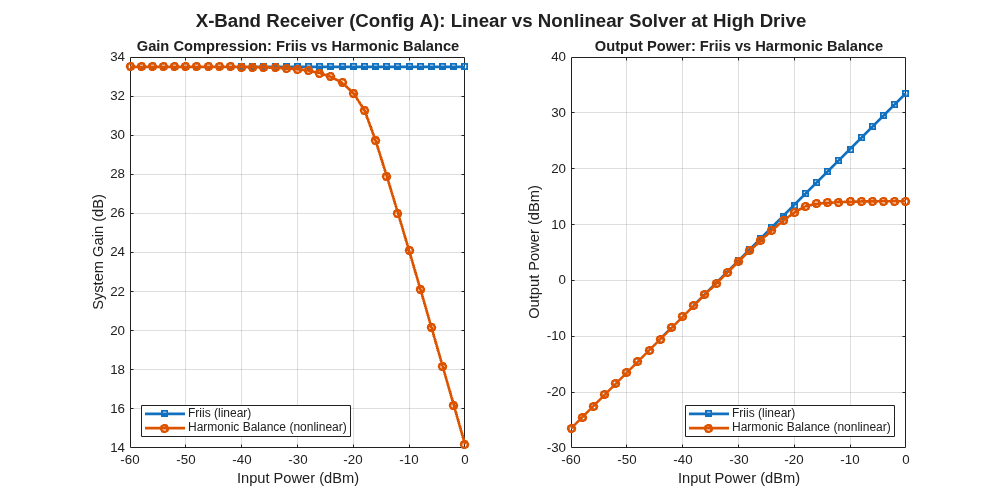
Find the approximate 1-dB compression point from the HB sweep. This is the input power at which the system gain drops by 1 dB from its small-signal value. The Friis solver cannot identify this point because it models constant gain at all power levels.
gainDrop = gainHB(1) - gainHB;
idx1dB = find(gainDrop >= 1, 1, 'first');
if ~isempty(idx1dB)
    fprintf('  HB-derived input P1dB ~ %.0f dBm  (gain drops from %.1f to %.1f dB)\n', ...
        sweepPowerComp(idx1dB), gainHB(1), gainHB(idx1dB));
    fprintf('  Friis gain at same power: %.1f dB  (no compression modeled)\n', ...
        gainFriis(idx1dB));
end
  HB-derived input P1dB ~ -20 dBm  (gain drops from 33.5 to 32.2 dB)
  Friis gain at same power: 33.5 dB  (no compression modeled)
Compute Link Budget and Dynamic Range
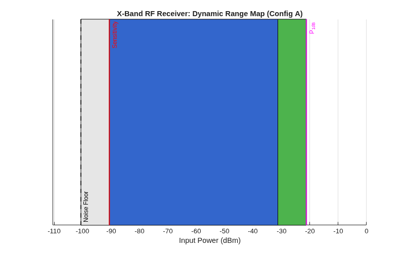
The link budget connects the receiver's RF performance to its operational capability. These derived metrics determine the receiver's ability to detect weak signals in the presence of strong interferers and quantify the usable input power range.
k_boltz = 1.38064852e-23;   % Boltzmann constant (J/K)
T0 = 290;                    % Reference temperature (K)
noiseFloor_W = k_boltz * T0 * spec.Bandwidth;
noiseFloor_dBm = 10*log10(noiseFloor_W) + 30;
sysNF = friisResult.NF(end);
effectiveFloor_dBm = noiseFloor_dBm + sysNF;
theoreticalSens = effectiveFloor_dBm + spec.RequiredSNR;
sysOIP3 = friisResult.OIP3(end);
sysGain = friisResult.TransducerGain(end);
outputNoiseFloor = effectiveFloor_dBm + sysGain;
sysIIP3 = friisResult.IIP3(end);

txt = [ ...
    "=================================================================" ; ...
    "  X-BAND LINK BUDGET AND DYNAMIC RANGE" ; ...
    "=================================================================" ; ...
    "" ; ...
    "  --- Thermal Noise Floor ---" ; ...
    sprintf("  kTB = %.2f dBm  (T=%.0f K, B=%.0f MHz)", noiseFloor_dBm, T0, spec.Bandwidth/1e6) ; ...
    sprintf("  System NF (Config A) = %.2f dB", sysNF) ; ...
    sprintf("  Effective noise floor = kTB + NF = %.2f dBm", effectiveFloor_dBm) ; ...
    "" ; ...
    "  --- Receiver Sensitivity ---" ; ...
    "  Sensitivity = kTB + NF + SNR_req" ; ...
    sprintf("             = %.2f + %.2f + %.0f", noiseFloor_dBm, sysNF, spec.RequiredSNR) ; ...
    sprintf("             = %.2f dBm", theoreticalSens) ; ...
    sprintf("  Spec target: %.0f dBm", spec.Sensitivity) ];
if theoreticalSens <= spec.Sensitivity
    txt = [txt ; sprintf("  Result: PASS (%.1f dB margin)", spec.Sensitivity - theoreticalSens)];
else
    txt = [txt ; sprintf("  Result: FAIL (%.1f dB short)", theoreticalSens - spec.Sensitivity)];
end

txt = [txt ; "" ; "  --- Spurious-Free Dynamic Range (SFDR) ---"];
if ~isinf(sysOIP3)
    sfdr = (2/3) * (sysOIP3 - outputNoiseFloor);
    txt = [txt ; ...
        sprintf("  OIP3 = %.2f dBm", sysOIP3) ; ...
        sprintf("  Output noise floor = %.2f dBm", outputNoiseFloor) ; ...
        "  SFDR = (2/3)(OIP3 - Output Noise Floor)" ; ...
        sprintf("       = (2/3)(%.2f - (%.2f))", sysOIP3, outputNoiseFloor) ; ...
        sprintf("       = %.2f dB", sfdr) ];
end

txt = [txt ; "" ; "  --- Estimated 1-dB Compression Point ---"];
if ~isinf(sysIIP3)
    p1dB_in = sysIIP3 - 9.6;
    p1dB_out = p1dB_in + sysGain;
    txt = [txt ; ...
        sprintf("  IIP3 = %.2f dBm", sysIIP3) ; ...
        sprintf("  Input P1dB  ~ IIP3 - 9.6 = %.2f dBm", p1dB_in) ; ...
        sprintf("  Output P1dB ~ %.2f dBm", p1dB_out) ];
end
txt = [txt ; "================================================================="];
disp(strjoin(txt, newline));
=================================================================
  X-BAND LINK BUDGET AND DYNAMIC RANGE
=================================================================

  --- Thermal Noise Floor ---
  kTB = -103.98 dBm  (T=290 K, B=10 MHz)
  System NF (Config A) = 3.38 dB
  Effective noise floor = kTB + NF = -100.59 dBm

  --- Receiver Sensitivity ---
  Sensitivity = kTB + NF + SNR_req
             = -103.98 + 3.38 + 10
             = -90.59 dBm
  Spec target: -90 dBm
  Result: PASS (0.6 dB margin)

  --- Spurious-Free Dynamic Range (SFDR) ---
  OIP3 = 21.89 dBm
  Output noise floor = -67.09 dBm
  SFDR = (2/3)(OIP3 - Output Noise Floor)
       = (2/3)(21.89 - (-67.09))
       = 59.32 dB

  --- Estimated 1-dB Compression Point ---
  IIP3 = -11.61 dBm
  Input P1dB  ~ IIP3 - 9.6 = -21.21 dBm
  Output P1dB ~ 12.29 dBm
=================================================================
Visualize the receiver's dynamic range as a horizontal bar chart. The map shows the noise floor, sensitivity threshold, spurious-free dynamic range (SFDR), and 1-dB compression point. The green region represents the usable input power range between sensitivity and compression.
figure('Name','X-Band Dynamic Range','Position',[400 100 800 500]);
hold on;
ypos = 0.5; barHeight = 0.3;

rectangle('Position',[effectiveFloor_dBm, ypos-barHeight/2, ...
    abs(effectiveFloor_dBm)+theoreticalSens, barHeight], ...
    'FaceColor',[0.9 0.9 0.9],'EdgeColor','k');

if ~isinf(sysIIP3)
    p1dB = sysIIP3 - 9.6;
    rectangle('Position',[theoreticalSens, ypos-barHeight/2, ...
        p1dB - theoreticalSens, barHeight], ...
        'FaceColor',[0.3 0.7 0.3],'EdgeColor','k');
    sfdrEnd = theoreticalSens + sfdr;
    if sfdrEnd > theoreticalSens && sfdrEnd < p1dB
        rectangle('Position',[theoreticalSens, ypos-barHeight/2, ...
            sfdr, barHeight], ...
            'FaceColor',[0.2 0.4 0.8],'EdgeColor','k');
    end
    xline(theoreticalSens, '-r', 'Sensitivity', 'LineWidth', 2, ...
        'LabelVerticalAlignment', 'top', 'FontSize', 9);
    xline(p1dB, '-m', 'P_{1dB}', 'LineWidth', 2, ...
        'LabelVerticalAlignment', 'top', 'FontSize', 9);
end
xline(effectiveFloor_dBm, '--k', 'Noise Floor', 'LineWidth', 1.5, ...
    'LabelVerticalAlignment', 'bottom', 'FontSize', 9);
hold off;
xlabel('Input Power (dBm)'); yticks([]);
title('X-Band RF Receiver: Dynamic Range Map (Config A)');
xlim([effectiveFloor_dBm - 10, 0]); grid on;
Summary
This example demonstrated a complete X-band receiver design workflow using rfbudget. The key findings are:
Component ordering is decisive. The LNA-first configuration (Config A) achieves a system NF several dB lower than the alternatives. At X-band, where component NFs are inherently higher, this advantage is even more critical than at lower frequencies.
The NF specification is the hardest to meet. All three configurations achieve sufficient gain and linearity, but only the LNA-first arrangement meets the strict 4 dB NF requirement.
The sensitivity sweep reveals operational impact. Config A maintains adequate SNR at input levels approximately 6-8 dB weaker than Config C, directly extending the receiver's usable sensitivity range.
IF filtering improves signal quality. Adding an IF bandpass filter after the mixer rejects mixer spurs and LO leakage without significantly degrading the system noise figure.
Harmonic Balance analysis provides a complete nonlinear picture. The HB solver reveals IP2 performance that the Friis solver cannot compute.
Compression exposes the Friis solver's limitation. The Friis solver reports constant gain regardless of input level, while the Harmonic Balance solver shows gain compression and output power saturation.
The link budget closes the loop. Computing sensitivity from first principles (kTB + NF + SNR_req), SFDR, and P1dB ensures the design meets all requirements across its full dynamic range.

