Develop Time Series Anomaly Detector in Time Series Anomaly Detector App

Time Series Anomaly Detector is an app that allows you to develop anomaly detectors that can detect abnormal patterns and points in data.

The app provides a graphical interface with which you can import both normal data and anomalous data.

Normal data, in this case, does not mean that the data set must be completely free of any anomalies. It just must be free of any anomalies with characteristics that you want to detect. This is because the training process considers all training data to represent normal behavior.

After importing your data, you can choose and train detectors, evaluate detection capability for different anomalies, and export the detector into your MATLAB^® workspace.

This tutorial shows how to develop a single time series anomaly detector, from data import to detector export.

Load Data and Open the App

Load training and anomaly data into your workspace using the following command.

load sineWaveAnomalyData

This data set includes a collection of time series that include both normal and abnormal behavior.

Open the app using the following command.

timeSeriesAnomalyDetector

Import Normal Data First for Training

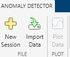
In the Anomaly Detector tab, in the File section, click Import data.

In the Select a data set to import dialog box, select sineWaveNormal only.

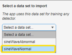
This data set contains ten members that each represent normal behavior. The app uses this data for training detectors throughout your session. The next dialog box shows the composition of the selected data.

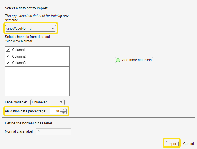
The data contains three channels and is unlabeled. In this dialog box, you also set the validation data percentage, which is the percentage of data that you hold back from the training process so that you can validate the training afterward. Click Import. The Data Sets pane now lists sineWaveNormal with a green dot to the left of it. The green dot indicates that this is the training data set.

Import Anomalous Data for Testing

Import the anomalous data by clicking Import Data once more.

In the Select additional data sets to import dialog box, select sineWaveAbnormal only.

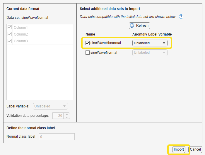
Leave sineWaveNormal unselected. The import dialog box always shows every data set variable in your workspace, including variables that you have already imported. If you import a data set the second time, the app creates a second independent copy of that data set.

Use Plot to Visualize the Normal and Abnormal Data

Visualize the data so that you can see the difference between the normal and abnormal data. To do so, In the Data Sets pane, select sineWaveNormal.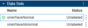

Then, in the Plot section of the Anomaly Detection tab, click Plot Data.

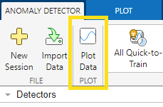
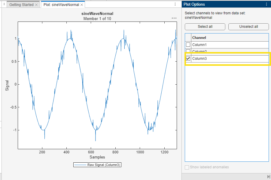
The app shows a plot of all three channels of the first member of the sineWaveNormal ensemble.

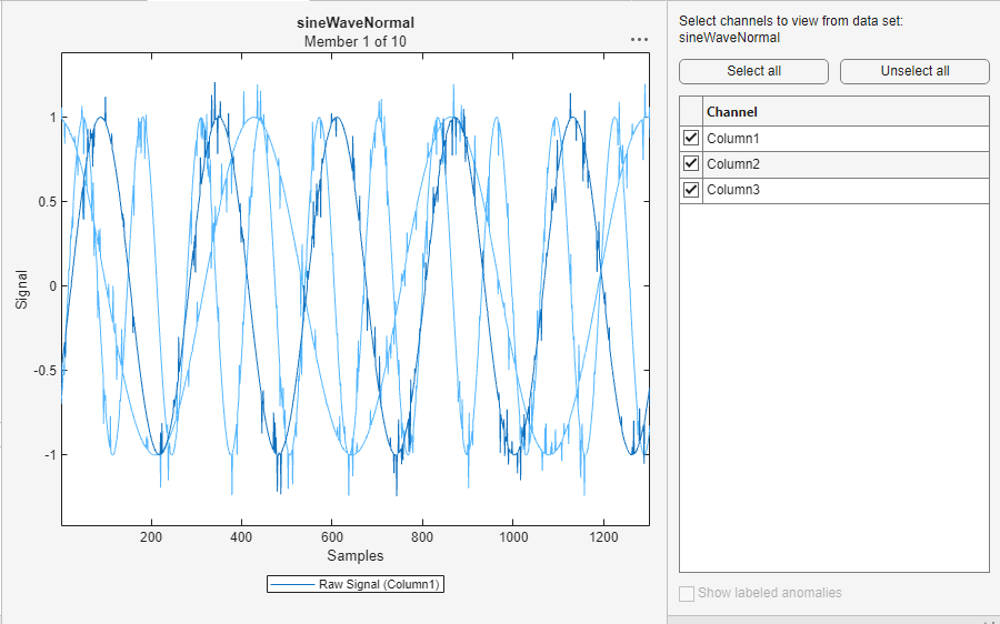
Isolate the third channel. Click Column 3 in the Plot Options pane. The plot now shows only Channel 3. All the channels look similar for the normal data. To change the member that you view, in the data section of the Anomaly Detector tab, choose a different member.

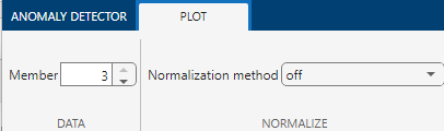
Visualize the abnormal data using the same process. Select sineWaveAbnormal and view all three channels together. You can isolate the channels in the same way as you isolated the channels of the normal data.

Choose a Detector

Choose a detector to start with. The Detectors section of the Anomaly Detector tab provides individual detectors and specific combinations of detectors.

A good way to begin exploring detectors is to start with detectors that are quicker to train. Click All Quick-to-Train.

The app adds these detectors in the Detectors pane. Each shows a status of draft, which means that the detector has not yet been trained. Select Isolation Forest.

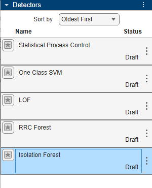
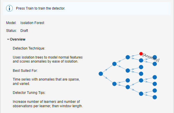
The app provides an overview of this detector, along with some guidance for tuning the detector to improve performance.

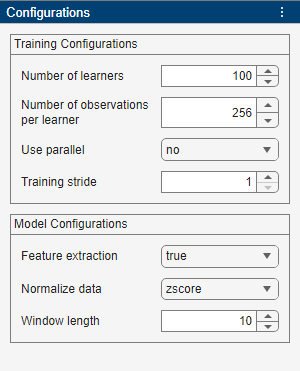
View the detector configuration. Currently, this dialog window shows the default training configuration.

Train Detector with Normal Data

Train the detector. First, click the Train section of the Anomaly Detector tab.

Note that Training Data Set lists sineWaveNormal. Then, in the Train section, click Train.

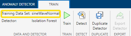
Notice that Training Data Set lists sineWaveNormal. Then, in the Train tab, click Train.

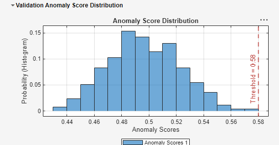
The app shows a histogram of the anomaly score distribution, with a vertical line representing the threshold on the right. This threshold is the border the bounds normal behavior from anomalous behavior when you perform detection.

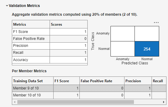
The metrics below the histogram show the aggregate validation metrics for the 20% training data holdback. In the confusion chart, all observations are classed as Normal.

It is worth noting that if your training data includes some anomalous behavior, that behavior will be classed as normal also, and will not be flagged as anomalous when you perform detection.

Test Detector with Abnormal Data

Now, test the trained detector using abnormal data. As the abnormal data plot showed previously, the abnormal data includes three members with three channels each. Each member contains a different anomaly, with a somewhat different signature for that anomaly across the three member channels.

In the Detect section of the Anomaly Detector tab, click Detect.

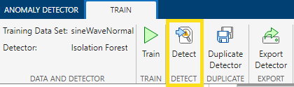
Then, in the Detect tab that appears, change Detection Data Set from sineWaveNormal to sineWaveAbnormal.

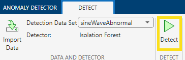
Click Detect. Then review the information in Detection Metrics.

The first and third members contain valid metrics describing the detector performance. The second member contains some NaNs.

Select Member 1 to review the member 1 results. First, view the detected anomalies plot. The red area indicates where the detector has detected anomalies.

The Anomaly Location table shows the anomaly locations within the time series along with the anomaly scores.

Now, view the anomaly scores for Member 1.

The plot shows the detections as they appear above the threshold. The threshold line cleanly separates the detected anomalies from the rest of the data.

View the same two plots for the third member.

The detector appears to perform well for the anomaly in member 3 as well.

Now view the results for member 2, and recall that the detector for this member did not show well-defined values in the detection metrics table.

You can see that for member 2, there are no anomaly detections at all. The threshold is higher than all the anomaly scores. This is why some of the metrics were not defined. This detector is capable of detecting the anomalies that members 1 and 3 contained, but in its current configuration, not capable of detecting the anomaly in member 2.

Export Trained Detector to MATLAB Workspace

Export the new anomaly detector to your MATLAB workspace. To do so, click the Export button in the Export section of the Anomaly Detector tab.

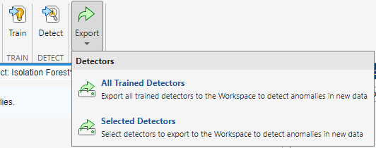
The Export menu lets you select whether to export all your models or a subset. If you select All Trained Detectors, the app immediately exports those detectors.

If you select Selected Detectors, the app shows a list of all trained detectors in the app. In this example, you have trained only one detector, so there is a single detector on the list.

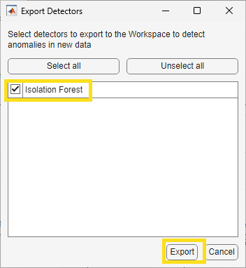
Click the Export button at the bottom of the selection dialog box. The detector is now in your MATLAB workspace with the name trainedDetector. View the properties of this detector in the command window.

trainedDetector = 

  TimeSeriesIForestDetector with properties:

                  NumLearners: 100
    NumObservationsPerLearner: 256
                  NumChannels: 3
                    IsTrained: 1
                 WindowLength: 10
               TrainingStride: 1
              DetectionStride: 10
                    Threshold: 0.5800
              ThresholdMethod: "kSigma"
           ThresholdParameter: 3
            ThresholdFunction: []
                Normalization: "zscore"
            FeatureExtraction: 1

You can now use this detector with other data sets, or continue to develop it at the command line.