Stencil Operations on a GPU

This example uses Conway's Game of Life to demonstrate how stencil operations can be performed using a GPU.

Many array operations can be expressed as a stencil operation, where each element of the output array depends on a small region of the input array. Examples include finite differences, convolution, median filtering, and finite-element methods. This example uses Conway's Game of Life to demonstrate two ways to run a stencil operation on a GPU, starting from the code in Cleve Moler's e-book Experiments in MATLAB.

In The Game of Life, cells are arranged in a 2-D grid. Each cell is in one of two states, referred to as living or dead, and the state of the cells evolves over a number of time steps. For each step, the state of each cell is determined by the state of its eight nearest neighbor:

Living cells die if they have if they have fewer than two neighbors.
Living cells die if they have more than three neighbors.
Dead cell become living if they have exactly three neighbors.
In all other configurations of, the state of the cell is unchanged.

This figure illustrates the rules. Only the state of the central cell and its eight neighbors are considered.

Generate a Random Initial Population

Create an initial population of cells on a 2-D grid with roughly 25% of the locations alive.

gridSize = 500;
initialGrid = (rand(gridSize) < .25);

Draw the initial grid

figure
imagesc(initialGrid)
colormap([1 1 1;0 0.5 0])
title("Initial Grid")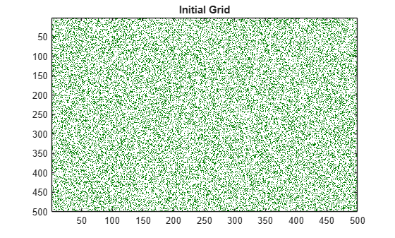

Define CPU Function

Define a function that updates the cells in the grid, based on the implementation in the e-book Experiments in MATLAB. This version is fully vectorized as it updates all cells in the grid in one pass per generation.

function X = updateGrid(X,N)
p = [1 1:N-1];
q = [2:N N];
% Count how many of the eight neighbors are alive.
neighbors = X(:,p) + X(:,q) + X(p,:) + X(q,:) + ...
    X(p,p) + X(q,q) + X(p,q) + X(q,p);
% A live cell with two live neighbors, or any cell with
% three live neighbors, is alive at the next step.
X = (X & (neighbors == 2)) | (neighbors == 3);
end

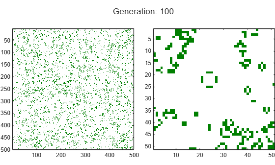
Run the Game of Life for 100 generations. Plot the entire grid and a 50-by-50 subset at each generation.

currentGrid = initialGrid;
numGenerations = 100;

figure
t = tiledlayout(1,2,TileSpacing="compact",Padding="tight");

gridAx = nexttile;
colormap([1 1 1;0 0.5 0]);
im = imagesc(gridAx,currentGrid);
axis square

zoomedAx = nexttile;
zoomedIm = imagesc(zoomedAx,currentGrid(50:100,50:100));
colormap([1 1 1;0 0.5 0]);
axis square

% Loop through each generation updating the grid and displaying it
for generation = 1:numGenerations
    currentGrid = updateGrid(currentGrid,gridSize);

    im.CData = currentGrid;
    zoomedIm.CData = currentGrid(50:100,50:100);
    title(t,"Generation: " + generation)
    drawnow
    pause(0.2)
end

Run the game for 1000 generations and measure how long it takes for each generation.

currentGrid = initialGrid;
numGenerations = 1000;

tic
for generation = 1:numGenerations
    currentGrid = updateGrid(currentGrid,gridSize);
end
cpuTime = toc;
fprintf('Average time on the CPU: %2.3f ms per generation.\n', ...
    1000*cpuTime/numGenerations);

Average time on the CPU: 2.971 ms per generation.

Convert the Game of Life to Run on a GPU

Run the Game of Life on the GPU by sending the initial grid to GPU memory using the gpuArray function. The algorithm remains unchanged. Use the wait function to ensure that the GPU has finished calculating before stopping the timer.

gpu = gpuDevice;
currentGrid = gpuArray(initialGrid);

tic
for generation = 1:numGenerations
    currentGrid = updateGrid(currentGrid,gridSize);
end

wait(gpu); % Only needed to ensure accurate timing
gpuSimpleTime = toc;

% Print out the average computation time and check the result is unchanged.
fprintf(['Average time on the GPU: %2.3f ms per generation ', ...
    '(%1.1fx faster).\n'], ...
    1000*gpuSimpleTime/numGenerations,cpuTime/gpuSimpleTime);

Average time on the GPU: 0.648 ms per generation (4.6x faster).

Create an Element-Wise Version for the GPU

The updateGrid function applies the same operations to each point in the grid independently. This suggests that arrayfun, which applies a function to each element of a gpuArray, could be used to do the evaluation. However, each cell needs to know about its eight neighbors, breaking the element-wise independence. In other words, each element needs to be able to access the full grid while also working independently.

The solution is to use a nested function. Nested functions, even those used with arrayfun, can access variables declared in their parent function. This means that each cell can read the whole grid from the previous time-step and index into it.

Define a function, updateGridArrayfun, that:

Defines a nested function, updateParentGrid, that updates a cell based on its own state and the state of its neighbors.
Applies the nested function using arrayfun.

By using nested function, the updateParentGrid function is able to access the grid variable even though it is not passed as an input argument.

function grid = updateGridArrayfun(grid,gridSize,numGenerations)

    function X = updateParentGrid(row,col,N)
        % Take account of boundary effects
        rowU = max(1,row-1);  rowD = min(N,row+1);
        colL = max(1,col-1);  colR = min(N,col+1);
        % Count neighbors
        neighbors ...
            = grid(rowU,colL) + grid(row,colL) + grid(rowD,colL) ...
            + grid(rowU,col)                   + grid(rowD,col) ...
            + grid(rowU,colR) + grid(row,colR) + grid(rowD,colR);
        % A live cell with two live neighbors, or any cell with
        % three live neighbors, is alive at the next step.
        X = (grid(row,col) & (neighbors == 2)) | (neighbors == 3);
    end

cols = gpuArray.colon(1,gridSize);
rows = cols';

for generation = 1:numGenerations
    grid = arrayfun(@updateParentGrid,rows,cols,gridSize);
end
end

initialGrid = gpuArray(initialGrid);

tic
currentGrid = updateGridArrayfun(initialGrid,gridSize,numGenerations);
wait(gpu); % Only needed to ensure accurate timing
gpuArrayfunTime = toc;

% Print out the average computation time and check the result is unchanged.
fprintf(['Average time using GPU arrayfun: %2.3fms per generation ', ...
    '(%1.1fx faster).\n'], ...
    1000*gpuArrayfunTime/numGenerations,cpuTime/gpuArrayfunTime);

Average time using GPU arrayfun: 0.369ms per generation (8.0x faster).

The function also uses another feature of arrayfun: dimension expansion. The function passes only the row and column vectors as input to arrayfun, which automatically expands them into the full grid. The effect is as though arrayfun calls the meshgrid function.

[cols,rows] = meshgrid(cols,rows);

This saves both computation and data transfer between CPU memory and GPU memory.

Conclusion

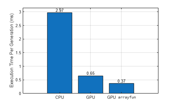
Compare the performance of the three methods.

figure
b = bar( ["CPU" "GPU" "GPU \fontname{monospace}arrayfun"], ...
    [1000*cpuTime/numGenerations 1000*gpuSimpleTime/numGenerations 1000*gpuArrayfunTime/numGenerations]);
ylabel("Execution Time Per Generation (ms)")
grid on
b(1).Labels = round(b(1).YData,2);

fprintf(['CPU:          %2.3f ms per generation.\n' ...
    'Simple GPU:   %2.3f ms per generation (%1.1fx faster).\n' ...
    'Arrayfun GPU: %2.3f ms per generation (%1.1fx faster).\n'], ...
    1000*cpuTime/numGenerations, ...
    1000*gpuSimpleTime/numGenerations,cpuTime/gpuSimpleTime, ...
    1000*gpuArrayfunTime/numGenerations,cpuTime/gpuArrayfunTime);

CPU:          2.971 ms per generation.
Simple GPU:   0.648 ms per generation (4.6x faster).
Arrayfun GPU: 0.369 ms per generation (8.0x faster).

In this example, you implement a simple stencil operation, Conway's Game of Life, on the GPU using arrayfun and variables declared in the parent function. You can also use this technique to access elements in a look-up table defined in the parent function.

When you apply the techniques described in this example to your own code, the performance improvement will strongly depend on your hardware and on the code you run.