Analyze Wind Data with Large Compute Cluster
This example shows how to access a large data set in the cloud and process it using hundreds of workers on a large cluster.
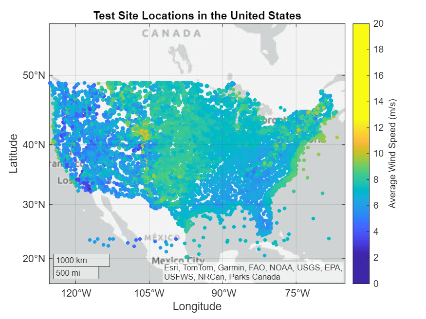
In this example, you use datastores and Parallel Computing Toolbox™ to conduct a wind resource assessment study of over 120,000 sites across the continental United States to find the best site for a wind farm.
The public data set in this example is part of the Wind Integration National Dataset Toolkit, or WIND Toolkit [1], [2], [3], [4]. For more information, see Wind Integration National Dataset Toolkit. The WIND toolkit is stored in a public Amazon S3™ bucket that is authorized for public access, so you do not need to configure authentication. For best results, run this example from an Amazon® Web Service (AWS®) cloud cluster.
To access the remote input data, you must specify the geographic region of the bucket using environmental variables.
setenv("AWS_DEFAULT_REGION","us-west-2");
Create a parallel pool and attach the function files the workers need to the pool. Send the client environment variable to the workers.
numWorkers = 450;
c = parcluster("HPCProfile");
pool = parpool(c,numWorkers,EnvironmentVariables="AWS_DEFAULT_REGION", ...
    AttachedFiles=["windNCReader.m","findWindTurbineSite.m",mfilename("fullpath")]);
Starting parallel pool (parpool) using the 'HPCProfile' profile ...
Connected to parallel pool with 450 workers.
Use a FileDatastore to manage access to the remote WIND dataset.
To speed up this example, load the pre-prepared windSitesDs datastore. If you need to recreate the datastore objects, you can use the createWindSitesDatastore helper function attached to this example.
load("windSitesDs.mat","windSitesDs")
% windSitesDs = createWindSitesDatastore;
Check whether the workers can access the files in the S3 bucket then reset the datastore.
f = parfeval(@(ds) summary(read(ds)),1,windSitesDs);
testOut = fetchOutputs(f)
testOut = struct with fields:
              Time: [1×1 struct]
        wind_speed: [1×1 struct]
    wind_direction: [1×1 struct]
           density: [1×1 struct]
       temperature: [1×1 struct]
          pressure: [1×1 struct]
reset(windSitesDs);
Process Site Data
Prepare Geographic Scatter Plot to Track Computations
Preallocate a table to collect progress summaries. The initializeGeoScatter helper function initializes a geographic scatter plot to visualize the different test locations and prepares settings such as title, labels, and limits.
itbl = table(size=[0,5],VariableTypes=["single","string","single","single","single"], ...
    VariableNames=["SiteID","ValueStoreKey","Latitude","Longitude","AvgWindSpeed"]);
s = initializeGeoScatter(itbl);

Set Up DataQueue to Track Progress
Create a DataQueue object to send progress summaries from the workers to the client. Use the afterEach function to define a callback on the client that updates the geographic scatter plot each time a worker sends the progress of a computation.
d = parallel.pool.DataQueue;
afterEach(d,@(x) updateGeoPlot(s,x));
Perform Computations and Update Progress
Prepare a parfor-loop to process the files in the datastore independently.
Inside the parfor-loop, partition the datastore based on the number of workers in the parallel pool. Initialize a cell array to store the progress data and specify the number of files to process before the workers send the progress data to the client. Then, read and analyze data from each file in the datastore using the findWindTurbine helper function attached to this example.
np = numpartitions(windSitesDs,pool);
parfor a = 1:np
    ds = partition(windSitesDs,np,a);
    updateSize = 12;
    geoTblUpdate = cell(updateSize,5);
    store = getCurrentValueStore;
    count = 0
    updateCount = 0

    while hasdata(ds)
        count = count+1;
        updateCount = updateCount+1;
        t = read(ds);
        results = findWindTurbineSite(t);
Store the results in the pool's ValueStore object. You can use the ValueStore when the combined size of all the results is large, or if the client requires the results during the parfor-loop. Otherwise, if your data is small or not required within the parfor block, the parfor output typically offers faster performance.
        key = strcat("set_",num2str(a)," result_",num2str(count));
        store(key) = results;
Collect the progress summary for each iteration.
        geoTblUpdate(updateCount,:) = {results.siteMetadata.siteID, ...
            key, ...
            results.siteMetadata.latitude, ...
            results.siteMetadata.longitude, ...
            results.overallData.wind_speed.Avg};
You can specify how often you want to send data back to the client. After processing 12 files, send the collected site information and preliminary results to the client.
        if updateCount >= updateSize
            send(d,geoTblUpdate);
            updateCount = 0;
            geoTblUpdate = cell(updateSize,5);
        end
    end
    if updateCount > 0
        send(d,geoTblUpdate(1:updateCount,:));
        updateCount = 0;
        geoTblUpdate = {};
    end
end
Perform Post-Processing Analysis
You can now interactively access the results in the pool's ValueStore. Using the ValueStore in this example is efficient because you keep the data on the cluster storage until you delete the parallel pool. This eliminates the need to transfer the data to and from the client during post data analysis. Such transfers can incur data overheads, especially with large amounts of data or on a network with high latency.
Use another parfor-loop to perform a post-analysis reduction operation to find the site that generates the maximum power.
clientStore = pool.ValueStore;
keySet = keys(clientStore);
maxPowerAndKey = cell(1,2);
parfor k = 1:length(keySet)
    store = getCurrentValueStore;
    key = keySet(k);
    results = store(key);
    maxPower = results.powerResults.maxPower;
    maxPowerAndKey = compareValue(maxPowerAndKey,{maxPower,key});
end
disp(maxPowerAndKey)
{[1.5374]} {["set_1534 result_5"]}
key = maxPowerAndKey{2};
bestSite = clientStore(key);
Summary of Promising Site Statistics
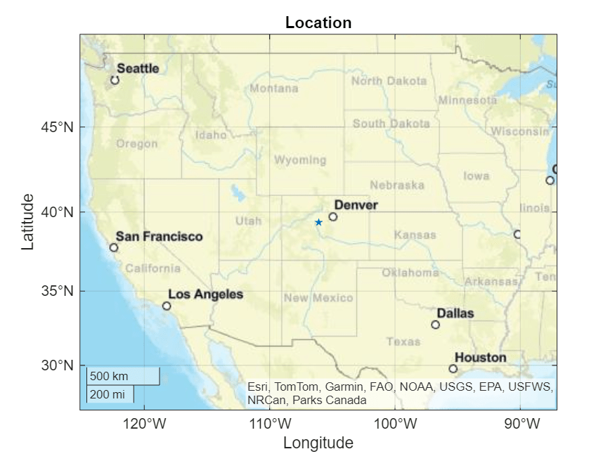
View a summary of the predicted best site for a wind farm.
Site Information
fprintf("Site ID: %d",bestSite.siteMetadata.siteID)Site ID: 47084
figure;
geoscatter(bestSite.siteMetadata.latitude,bestSite.siteMetadata.longitude,"pentagram","filled");
title("Location")
geobasemap streets

Wind Statistics
fprintf("Mean Wind Speed (m/s): %3.2f\n" + ...
    "Std. Dev. of Wind Speed (m/s): %3.2f\n" + ...
    "Max. Wind Speed (m/s): %3.2f\n", ...
    bestSite.overallData.wind_speed.Avg,bestSite.overallData.wind_speed.StdDev,bestSite.overallData.wind_speed.Max);
Mean Wind Speed (m/s): 11.56
Std. Dev. of Wind Speed (m/s): 5.06
Max. Wind Speed (m/s): 36.73
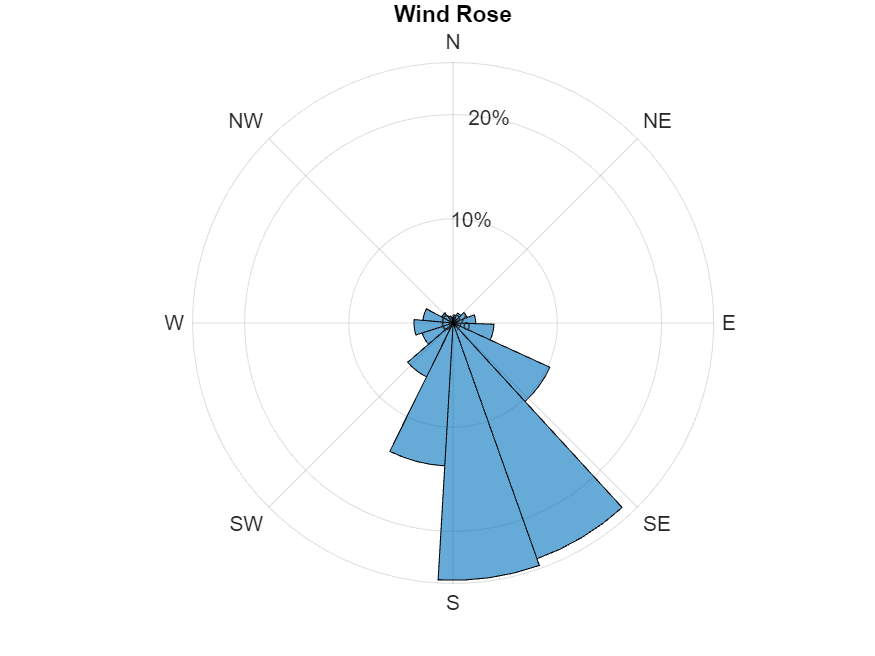
Display the wind direction distribution in a wind rose plot.
figure;
h = polarhistogram("BinEdge",bestSite.windDirectionHist.edges,"BinCounts",bestSite.windDirectionHist.counts);
pax = gca;
pax.ThetaZeroLocation = "top";
pax.ThetaDir = 'clockwise';
pax.ThetaTick = 0:45:360;
pax.ThetaTickLabel = ["N","NE","E","SE","S","SW","W","NW"];
pax.RTickLabel = num2str(str2double(pax.RTickLabel)*100)+"%";
title("Wind Rose")

Display a summary of the annual power, capacity factor and annual energy production for each class of wind turbine.
disp(bestSite.powerResults.summary)
    Turbine Class    Turbine Rated Power (MW)    Averaged Power (kW)    Capacity Factor (%)    Annual Energy Production (MWh)
    _____________    ________________________    ___________________    ___________________    ______________________________

          1                     2                      1443.4                 72.171                       12644
          2                     2                      1537.4                 76.871                       13468
          3                     2                      1518.2                 75.911                       13300
After you have finished analyzing the results data, you can delete the parallel pool. Deleting the parallel pool also deletes the data in the ValueStore so if you want to preserve the data, copy the data in the ValueStore to another location before deleting the pool.
delete(pool);
Local Functions
The initializeGeoScatter function initializes a geographic scatter plot you use to display updates from the workers.
function s = initializeGeoScatter(itbl)
    s = geoscatter(itbl,"Latitude","Longitude",ColorVariable="AvgWindSpeed",SizeData=10,MarkerFaceColor="flat");
    c = colorbar;
    c.Label.String = "Average Wind Speed (m/s)";
    c.Limits = [0,20];
    title("Test Site Locations in the United States");
    geolimits([25 50],[-125.4 -65.0]);
end
The compareValue function determines which of the two input cell arrays contains the greater numerical value at the first position and returns the corresponding cell array.
function v = compareValue(currentMaxPower,candidate)
    valueA = currentMaxPower{1};
    valueB = candidate{1};
    if valueA > valueB
        v = currentMaxPower;
    else
        v = candidate;
    end
end
The updateGeoPlot function updates the geographic scatter plot when a worker sends new data to the client.
function updateGeoPlot(s,x)
    s.SourceTable = [s.SourceTable;x];
    drawnow limitrate nocallbacks;
end
References
[1] Draxl, Caroline, Bri-Mathias Hodge, Andrew Clifton, and Jim McCaa. "Overview and Meteorological Validation of the Wind Integration National Dataset Toolkit (Technical Report, NREL/TP-5000-61740)". Golden, CO: National Renewable Energy Laboratory (2015). https://www.nrel.gov/docs/fy15osti/61740.pdf
[2] Draxl, Caroline, Andrew Clifton, Bri-Mathias Hodge, and Jim McCaa. “The Wind Integration National Dataset (WIND) Toolkit.” Applied Energy 151 (August 2015): 355–66 https://doi.org/10.1016/j.apenergy.2015.03.121
[3] King, J., Andrew Clifton, and Bri-Mathias Hodge. "Validation of Power Output for the WIND Toolkit (Technical Report, NREL/TP-5D00-61714)". Golden, CO: National Renewable Energy Laboratory (2014). https://www.nrel.gov/docs/fy14osti/61714.pdf
[4] Lieberman-Cribbin, W., Caroline Draxl, and Andrew Clifton. "Guide to Using the WIND Toolkit Validation Code (Technical Report, NREL/TP-5000-62595)". Golden, CO: National Renewable Energy Laboratory (2014). https://www.nrel.gov/docs/fy15osti/62595.pdf
See Also
Scale Up Parallel Code to Large Clusters