Visualize Aircraft Line-of-Sight over Terrain

R2026b

Since R2026b

This example shows how to compute and visualize the line-of-sight (LOS) visibility of an aircraft from a ground location over terrain. First, import terrain data for a region and apply it to a 3D scenario. Then, perform point-to-point visibility analysis from a ground location to a simulated flight path, and display the results using a 3D scenario viewer. Finally, perform point-to-area visibility analysis from the ground location for an aircraft flying at constant altitude, and display the results on a 2D geographic axes.

Use LOS analysis for ground-to-air scenarios where unobstructed visibility is important, such as for radar surveillance, communications, and UAV path planning. This example applies the analysis to radar surveillance for an airport.

Import Terrain Data

Specify a DTED-format terrain file to use for data analysis and 3D visualization. The terrain file is from the SRTM Void Filled data set from the United States Geological Survey (USGS).

dtedfile = "n39_w106_3arc_v2.dt1";
attribution = "SRTM 3 arc-second resolution. Data available from the U.S. Geological Survey.";

Import the DTED data into the workspace as an array and a geographic raster reference object. Prepare to use the data with analysis functions by specifying the return type as "double".

[Zterrain,Rterrain] = readgeoraster(dtedfile,OutputType="double");

Query the geographic limits and the sample resolution of the DTED data by accessing properties of the reference object. The limits for the file correspond to a region around Boulder, Colorado, US. The resolution corresponds to the DTED level-1 format, which has sample resolution of 3 arc seconds, or about 90 meters.

latlim = Rterrain.LatitudeLimits;
lonlim = Rterrain.LongitudeLimits;
latspc = Rterrain.SampleSpacingInLatitude;
lonspc = Rterrain.SampleSpacingInLongitude;
disp("Latitude limits of terrain: " + mat2str(latlim) + newline + ...
    "Longitude limits of terrain: " + mat2str(lonlim) + newline + ...
    "Terrain resolution in latitude: " + latspc*3600 + " arc seconds" + newline + ...
    "Terrain resolution in longitude: " + lonspc*3600 + " arc seconds")

Latitude limits of terrain: [39 40]
Longitude limits of terrain: [-106 -105]
Terrain resolution in latitude: 3 arc seconds
Terrain resolution in longitude: 3 arc seconds

Visualize Aircraft Trajectory LOS in 3D Scenario Viewer

Perform point-to-point LOS analysis from a radar location to a points along an aircraft trajectory. Visualize the analysis in a 3D scenario viewer.

Create 3D Scenario and Viewer with Custom Terrain

Add custom terrain data from a DTED file. If custom terrain called "southboulder" already exists, avoid overwriting the terrain by specifying NameExistsRule as "preserve".

addCustomTerrain("southboulder",dtedfile,NameExistsRule="preserve",Attribution=attribution)

Create a 3D scenario that uses the custom terrain data. Display the scenario in a viewer.

scnro = scenario(Terrain="southboulder");
v = viewer(scnro);

View Radar Ground Location

Define a radar ground location at Rocky Mountain Metropolitan Airport. The radar is mounted on a tower 10 meters above the ground.

rdrlat = 39.913756;
rdrlon = -105.118062;
rdrtowerht = 10;
rdrpos = pointtable(rdrlat,rdrlon,rdrtowerht,HeightReference="terrain");

Add the radar to the scenario by creating a generic point actor. When you add an actor to a scenario, the scenario automatically creates a visual in the viewer. Set the color of the visual to cyan.

rdr = actor(scnro,rdrpos);
rdr.Visual.MarkerFaceColor = "cyan";

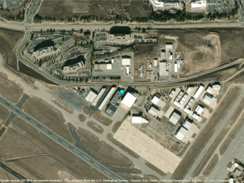
View the radar from 1 km overhead.

follow(v,rdr,Offset=[0 0 1000])

Simulate Aircraft Trajectory

Simulate the trajectory of an aircraft circling over the mountains.

Define the center point of the circular path.

tlat0 = 39.80384;
tlon0 = -105.49916;
tht0 = 3000;

Define the waypoints for the trajectory using east-north-up (ENU) Cartesian coordinates. Specify the coordinates of a curve with a radius of 5 km and a vertical climb of 1 km over 1.5 revolutions. Then, convert the ENU coordinates to geodetic coordinates that are referenced to the WGS84 ellipsoid.

azs = 1:540;
r = 5000; % 5 km
[X,Y] = pol2cart(deg2rad(azs),r);
Z = linspace(0,1000,numel(azs)); % 1 km
[tlat,tlon,tht] = enu2geodetic(X,Y,Z,tlat0,tlon0,tht0,wgs84Ellipsoid);

Create an air trajectory from the waypoints.

waypoints = pointtable(tlat,tlon,tht,HeightReference="ellipsoid");
traj = airTrajectory(waypoints,GroundSpeed=110); % ~250 mph

Add an aircraft actor to the scenario. Specify the trajectory of the aircraft using the air trajectory.

ac = aircraft(scnro,traj);
follow(ac)

When you add an actor to a scenario, the scenario automatically creates a visual in the viewer. Hide the waypoint markers in the visual.

trajvis = ac.Behavior.Visual;
trajvis.ShowWaypoints = false;

Set the time step of the aircraft in the simulation to 0.5 seconds.

ac.Behavior.TimeStep = seconds(0.5);

View Aircraft Trajectory over Terrain

View the 3D terrain and the radar from a distance by changing the camera position and rotation angles.

campt = pointtable(39.77114,-105.62662,6670,HeightReference="ellipsoid");
campos(v,campt)
camheading(v,70)
campitch(v,-12)
camroll(v,0)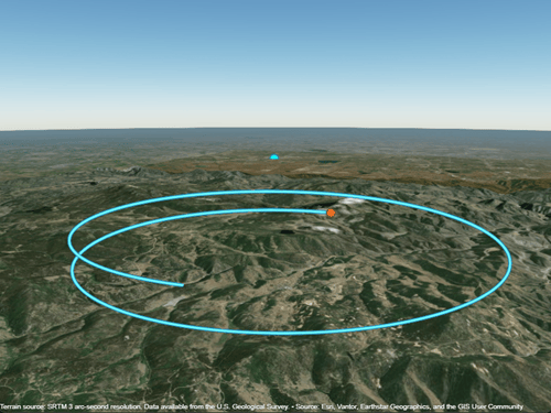

Create LOS Analysis with Aircraft

Create an LOS analysis between the radar and aircraft. The LOS calculation does not account for refraction through the atmosphere.

losA = losAnalysis(rdr,ac);

When you add an analysis to a scenario, the scenario automatically creates a visual in the viewer. Set the color of the obstructed line to magenta.

losvis = losA.Visual;
losvis.ObstructedColor = "magenta";

Simulate and Visualize LOS Visibility over Terrain

Simplify the visualization by hiding the trajectory visual.

trajvis.Visible = false;

Run the simulation. Each time the scenario advances, compute and display the LOS visibility. Display green markers where the aircraft is visible and magenta markers where it is not visible. For the first half of the simulation, view the scene from a distance. For the second half of the simulation, follow the aircraft.

following = false;
while advance(scnro)
    % Compute visibility
    isvis = hasLOS(losA);

    % Display marker color-coded by visibility
    if isvis
        clr = losvis.VisibleColor;
    else
        clr = losvis.ObstructedColor;
    end
    acpos = position(ac);
    plotpoints(v,acpos,MarkerSize=3,MarkerFaceColor=clr,MarkerEdgeColor=clr);

    % Follow the aircraft in second half of simulation
    if ~following && scnro.SimulationTime > seconds(235)
        follow(ac);
    end
end

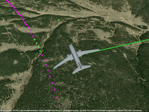
Hide the visual associated with the LOS analysis. Then, restore the view of the 3D terrain and the radar from a distance.

losvis.Visible = false;

campos(v,campt)
camheading(v,70)
campitch(v,-12)
camroll(v,0)

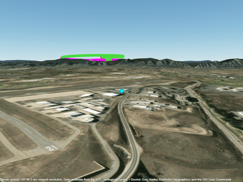
View the LOS analysis visual from the perspective of the radar. Specify the camera offset as 900 meters east, 200 meters north, and 100 meters up from the radar location. Note that the green markers are visible, but the magenta markers are either completely or partially obstructed by the terrain.

follow(rdr,Offset=[900 200 100])

Visualize Aircraft LOS Visibility Contours on 2D Map

The previous sections performed point-to-point LOS analysis and visualization from a radar location to an aircraft trajectory. This time, perform point-to-area LOS analysis and visualization from the same radar location across the terrain region. The visualization displays the edge of visibility for an aircraft flying at constant altitude.

Plot Radar Location and Terrain Limits on a 2D Map

Display the radar location in a 2D map that uses a topographic basemap.

figure
geoplot(rdrlat,rdrlon,"co",MarkerSize=3,LineWidth=6,DisplayName="Radar location")
geobasemap topographic
gx = gca;
gx.MapLayout = "maximized";

Visualize the boundary of the custom terrain by displaying an area of interest (AOI) on the map.

aoi = aoiquad(latlim,lonlim);
hold on
geoplot(aoi,LineWidth=1,FaceColor="none",DisplayName="Terrain limits")

Add a legend in the northwest corner.

legend(Location="northwest")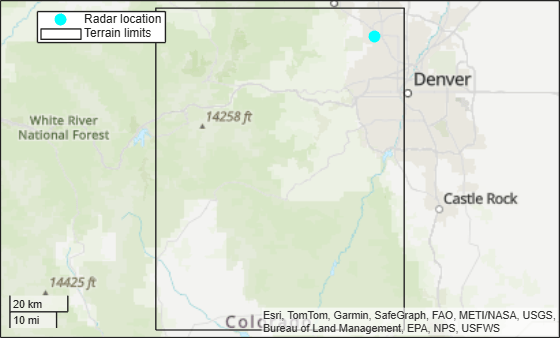

Plot Visibility Contours for Aircraft Flying at Constant Altitude

Specify three altitudes above mean sea level for the aircraft. For each altitude:

• Compute the viewshed using the radar location as the observer. The viewshed defines the area that has LOS visibility.

• Find the edge of aircraft visibility by computing contours from the viewshed data.

• Remove small contour segments.

• Plot the contours on the 2D map.

tgtalts = [3000 4000 5000];

minVertices = 10;
cfig = figure(Visible="off"); % Suppress contour plot using invisible figure
cax = axes(Parent=cfig);

rdralt = 1717 + rdrtowerht;
for tgtalt = tgtalts
    vis = viewshed(Zterrain,Rterrain,rdrlat,rdrlon,rdralt,tgtalt,"MSL","MSL");
    
    C = contourm(vis,Rterrain,LevelList=1,Parent=cax);
    clat = C(2,:);
    clon = C(1,:);
    
    clats = [];
    clons = []; 
    k = 1;   
    while k < size(C,2)
        numVertices = clat(k);
        if numVertices > minVertices % Do not plot small segments 
            clats = [clats clat(k+1:k+numVertices) NaN]; %#ok<AGROW> 
            clons = [clons clon(k+1:k+numVertices) NaN]; %#ok<AGROW> 
        end
        k = k + numVertices + 1;
    end
    
geoplot(gx,clats,clons,LineWidth=2,DisplayName="Aircraft: " + string(tgtalt) + " m");
end

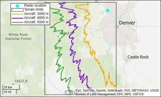
The contours appear primarily to the west of the radar. The contours do not appear in other directions because terrain does not obstruct visibility in those directions within the terrain limits.

Where the LOS visibility of the radar is obstructed, the contours correspond to radar coverage regions for three altitudes. The contour nearest to the radar corresponds to radar coverage for an aircraft flying at 3000 meters, and the contour farthest from the radar corresponds to radar coverage for an aircraft flying at 5000 meters.

The viewshed function calculates LOS visibility by assuming the data is referenced to a spherical Earth. However, the data is actually referenced to the WGS84 ellipsoid. As a result, there can be minor discrepancies. The LOS calculation also corresponds to optical LOS and does not account for refraction through the atmosphere.