timeoptions
Create list of time plot options
Description
Use the timeoptions command to create a
TimeOptions object to customize time plot appearance. You can also use
the command to override the plot preference settings in the MATLAB® session in which you create the time plots.
Creation
Description
plotoptions = timeoptions
plotoptions = timeoptions('cstprefs')
Properties
Object Functions
getoptions | Return plot options handle or plot options property |
impulseplot | Plot impulse response with additional plot customization options |
initialplot (Control System Toolbox) | Plot initial condition response with additional plot customization options |
lsimplot | Plot simulated time response of dynamic system to arbitrary inputs with additional plot customization options |
setoptions | Set plot options handle or plot options property |
stepplot | Plot step response with additional plot customization options |
Examples
Plot Normalized Step Response
Create a default time options set.
opt = timeoptions;
Enable plotting of normalized responses.
opt.Normalize = 'on';Plot the step response of two transfer function models using the specified options.
sys1 = tf(10,[1,1]);
sys2 = tf(5,[1,5]);
stepplot(sys1,sys2,opt);
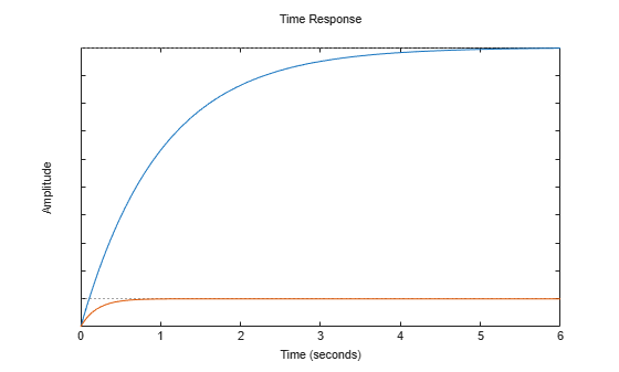
The plot shows the normalized step response for the two transfer function models.
Customize Step Plot using Plot Handle
For this example, use the plot handle to change the time units to minutes and turn on the grid.
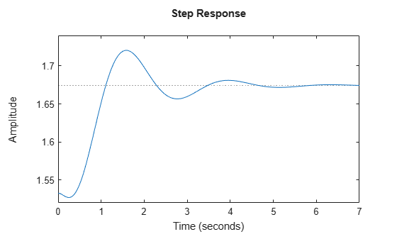
Generate a random state-space model with 5 states and create the step response plot with plot handle h.
rng("default")
sys = rss(5);
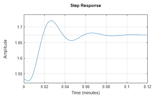
h = stepplot(sys);Change the time units to minutes and turn on the grid. To do so, edit properties of the plot handle, h using setoptions.
setoptions(h,'TimeUnits','minutes','Grid','on');
The step plot automatically updates when you call setoptions.
Alternatively, you can also use the timeoptions command to specify the required plot options. First, create an options set based on the toolbox preferences.
plotoptions = timeoptions('cstprefs');Change properties of the options set by setting the time units to minutes and enabling the grid.
plotoptions.TimeUnits = 'minutes';
plotoptions.Grid = 'on';
stepplot(sys,plotoptions);
You can use the same option set to create multiple step plots with the same customization. Depending on your own toolbox preferences, the plot you obtain might look different from this plot. Only the properties that you set explicitly, in this example TimeUnits and Grid, override the toolbox preferences.
Customized Step Response Plot at Specified Time
For this example, examine the step response of the following zero-pole-gain model and limit the step plot to tFinal = 15 s. Use 15-point blue text for the title. This plot should look the same, regardless of the preferences of the MATLAB session in which it is generated.
sys = zpk(-1,[-0.2+3j,-0.2-3j],1)*tf([1 1],[1 0.05]);
tFinal = 15;
First, create a default options set using timeoptions.
plotoptions = timeoptions;
Next change the required properties of the options set plotoptions.
plotoptions.Title.FontSize = 15;
plotoptions.Title.Color = [0 0 1];
Now, create the step response plot using the options set plotoptions.
h = stepplot(sys,tFinal,plotoptions);
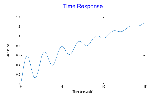
Because plotoptions begins with a fixed set of options, the plot result is independent of the toolbox preferences of the MATLAB session.
Custom Plot of System Evolution from Initial Condition
By default, lsimplot simulates the model assuming all states are zero at the start of the simulation. When simulating the response of a state-space model, use the optional x0 input argument to specify nonzero initial state values. Consider the following two-state SISO state-space model.
A = [-1.5 -3;
      3   -1];
B = [1.3; 0];
C = [1.15 2.3];
D = 0;
sys = ss(A,B,C,D);
Suppose that you want to allow the system to evolve from a known set of initial states with no input for 2 s, and then apply a unit step change. Specify the vector x0 of initial state values, and create the input vector.
x0 = [-0.2 0.3];
t = 0:0.05:8;
u = zeros(length(t),1);
u(t>=2) = 1;
First, create a default options set using timeoptions.
plotoptions = timeoptions;
Next change the required properties of the options set plotoptions and plot the simulated response with the zero order hold option.
plotoptions.Title.FontSize = 15;
plotoptions.Title.Color = [0 0 1];
plotoptions.Grid = 'on';
h = lsimplot(sys,u,t,x0,plotoptions,'zoh');
hold on
title('Simulated Time Response with Initial Conditions')
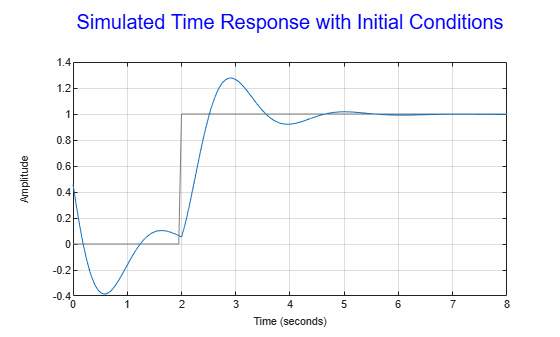
The first half of the plot shows the free evolution of the system from the initial state values [-0.2 0.3]. At t = 2 there is a step change to the input, and the plot shows the system response to this new signal beginning from the state values at that time. Because plotoptions begins with a fixed set of options, the plot result is independent of the toolbox preferences of the MATLAB session.
Customized Plot of Simulated Response to Arbitrary Input Signal
For this example, change time units to minutes and turn the grid on for the simulated response plot. Consider the following transfer function.
sys = tf(3,[1 2 3]);
To compute the response of this system to an arbitrary input signal, provide lsimplot with a vector of the times t at which you want to compute the response and a vector u containing the corresponding signal values. For instance, plot the system response to a ramping step signal that starts at 0 at time t = 0, ramps from 0 at t = 1 to 1 at t = 2, and then holds steady at 1. Define t and compute the values of u.
t = 0:0.04:8;
u = max(0,min(t-1,1));
Use lsimplot plot the system response to the signal with a plot handle h.
h = lsimplot(sys,u,t);
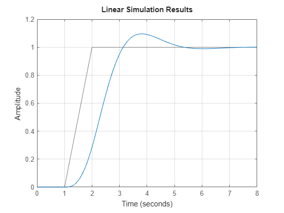
The plot shows the applied input (u,t) in gray and the system response in blue.
Use the plot handle to change the time units to minutes and to turn the grid on. To do so, edit properties of the plot handle, h using setoptions.
setoptions(h,'TimeUnits','minutes','Grid','on')
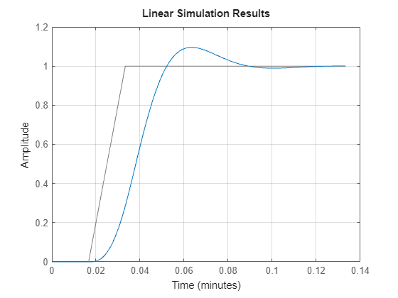
The plot automatically updates when you call setoptions.
Alternatively, you can also use the timeoptions command to specify the required plot options. First, create an options set based on the toolbox preferences.
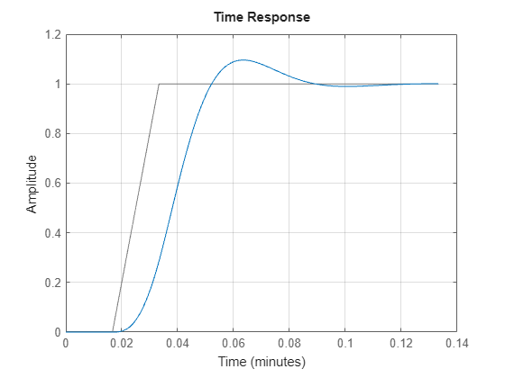
plotoptions = timeoptions('cstprefs');Change properties of the options set by setting the time units to minutes and enabling the grid.
plotoptions.TimeUnits = 'minutes';
plotoptions.Grid = 'on';
lsimplot(sys,u,t,plotoptions);
Version History
Introduced in R2012a
See Also
getoptions | impulseplot | initialplot (Control System Toolbox) | lsimplot | setoptions | stepplot
You can also select a web site from the following list:
Americas
- América Latina (Español)
- Canada (English)
- United States (English)
Europe
- Belgium (English)
- Denmark (English)
- Deutschland (Deutsch)
- España (Español)
- Finland (English)
- France (Français)
- Ireland (English)
- Italia (Italiano)
- Luxembourg (English)
- Netherlands (English)
- Norway (English)
- Österreich (Deutsch)
- Portugal (English)
- Sweden (English)
- Switzerland
- United Kingdom (English)