Plotting the Efficient Frontier for a PortfolioMAD Object

This example shows how to use the plotFrontier function creates a plot of the efficient frontier for a given portfolio optimization problem. This function accepts several types of inputs and generates a plot with an optional possibility to output the estimates for portfolio risks and returns along the efficient frontier. plotFrontier has four different ways that it can be used. In addition to a plot of the efficient frontier, if you have an initial portfolio in the InitPort property, plotFrontier also displays the return versus risk of the initial portfolio on the same plot. If you have a well-posed portfolio optimization problem set up in a PortfolioMAD object and you use plotFrontier, you get a plot of the efficient frontier with the default number of portfolios on the frontier (the default number is currently 10 and is maintained in the hidden property defaultNumPorts).

Create Efficient Frontier Plot

To plot the efficient frontier for a PortflioMAD object, use of plotFrontier.

m = [ 0.05; 0.1; 0.12; 0.18 ];
C = [ 0.0064 0.00408 0.00192 0; 
    0.00408 0.0289 0.0204 0.0119;
    0.00192 0.0204 0.0576 0.0336;
    0 0.0119 0.0336 0.1225 ];
m = m/12;
C = C/12;

AssetScenarios = mvnrnd(m, C, 20000);

p = PortfolioMAD;
p = setScenarios(p, AssetScenarios);
p = setDefaultConstraints(p);

plotFrontier(p)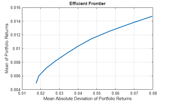

The Name property appears as the title of the efficient frontier plot if you set it in the PortfolioMAD object. Without an explicit name, the title on the plot would be "Efficient Frontier." If you want to obtain a specific number of portfolios along the efficient frontier, use plotFrontier with the number of portfolios that you want.

Suppose that you have this PortfolioMAD object and you want to plot 20 portfolios along the efficient frontier and to obtain 20 risk and return values for each portfolio:

[prsk, pret] = plotFrontier(p, 20);

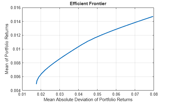
display([pret, prsk])

    0.0049    0.0175
    0.0054    0.0179
    0.0060    0.0189
    0.0065    0.0204
    0.0070    0.0223
    0.0075    0.0245
    0.0080    0.0270
    0.0085    0.0297
    0.0090    0.0325
    0.0096    0.0354
    0.0101    0.0384
    0.0106    0.0414
    0.0111    0.0447
    0.0116    0.0487
    0.0121    0.0531
    0.0127    0.0579
    0.0132    0.0630
    0.0137    0.0684
    0.0142    0.0739
    0.0147    0.0796

Plotting Existing Efficient Portfolios

If you already have efficient portfolios from any of the "estimateFrontier" functions (see Estimate Efficient Frontiers for PortfolioMAD Object), pass them into plotFrontier directly to plot the efficient frontier

m = [ 0.05; 0.1; 0.12; 0.18 ];
C = [ 0.0064 0.00408 0.00192 0; 
    0.00408 0.0289 0.0204 0.0119;
    0.00192 0.0204 0.0576 0.0336;
    0 0.0119 0.0336 0.1225 ];
m = m/12;
C = C/12;

AssetScenarios = mvnrnd(m, C, 20000);

pwgt0 = [ 0.3; 0.3; 0.2; 0.1 ];

p = PortfolioMAD('Name', 'Asset Allocation Portfolio', 'InitPort', pwgt0);

p = setScenarios(p, AssetScenarios);
p = setDefaultConstraints(p);

pwgt = estimateFrontier(p, 20);
plotFrontier(p, pwgt)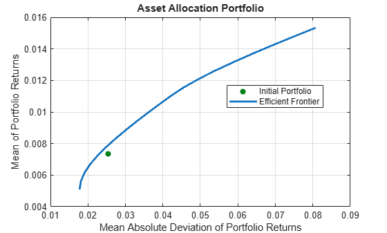

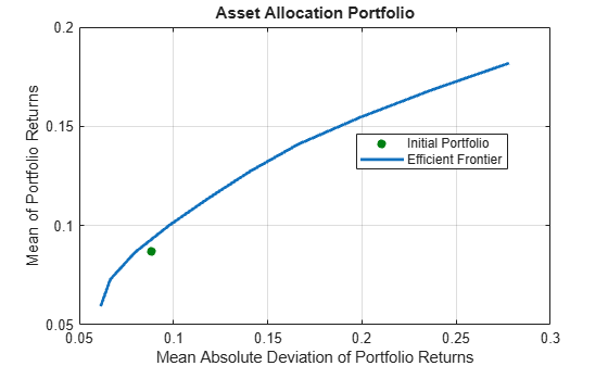
Plotting Existing Efficient Portfolio Risks and Returns

If you already have efficient portfolio risks and returns, you can use the interface to plotFrontier to pass them into plotFrontier to obtain a plot of the efficient frontier:

m = [ 0.05; 0.1; 0.12; 0.18 ];
C = [ 0.0064 0.00408 0.00192 0; 
      0.00408 0.0289 0.0204 0.0119;
      0.00192 0.0204 0.0576 0.0336;
      0 0.0119 0.0336 0.1225 ];

AssetScenarios = mvnrnd(m, C, 20000);

pwgt0 = [ 0.3; 0.3; 0.2; 0.1 ];

p = PortfolioMAD('Name', 'Asset Allocation Portfolio', 'InitPort', pwgt0);

p = setScenarios(p, AssetScenarios);
p = setDefaultConstraints(p);

pwgt = estimateFrontier(p);

pret= estimatePortReturn(p, pwgt)

pret = 10×1

    0.0592
    0.0729
    0.0865
    0.1001
    0.1137
    0.1274
    0.1410
    0.1546
    0.1682
    0.1819

prsk = estimatePortRisk(p, pwgt)

prsk = 10×1

    0.0614
    0.0665
    0.0796
    0.0978
    0.1185
    0.1407
    0.1662
    0.1992
    0.2367
    0.2781

plotFrontier(p, prsk, pret)