getLoopTransfer
Open-loop transfer function of control system represented by
genss model
Syntax
Description
L = getLoopTransfer(T,Locations)T, containing the analysis points specified
by Locations. The point-to-point open-loop transfer function is
the response obtained by opening the loop at the specified locations, injecting
signals at those locations, and measuring the return signals at the same locations.
Examples
Open-Loop Transfer Function at Analysis Point
Compute the open-loop response of the following control system model at an analysis point specified by an AnalysisPoint block, X.
![]()
Create a model of the system by specifying and connecting a numeric LTI plant model, G, a tunable controller, C, and the AnalysisPoint, X.
G = tf([1 2],[1 0.2 10]);
C = tunablePID('C','pi');
X = AnalysisPoint('X');
T = feedback(G*X*C,1);
T is a genss model that represents the closed-loop response of the control system from to . The model contains AnalysisPoint block X, which identifies the potential loop-opening location.
Calculate the open-loop point-to-point loop transfer at location X.
L = getLoopTransfer(T,'X');This command computes the transfer function you would obtain by opening the loop at X, injecting a signal into G, and measuring the resulting response at the output of C. By default, getLoopTransfer computes the positive feedback transfer function, which is the loop transfer assuming that the loop will be closed at X without a change of sign. In this example, the positive feedback transfer function is .
The output L is a genss model that includes the tunable block C. You can use getValue to obtain the current value of L, in which all the tunable blocks of L are evaluated to their current numeric value.
Stability Margins of Closed-Loop System
Compute the stability margins of the following closed-loop system at an analysis point specified by an AnalysisPoint block, X.
![]()
Create a model of the system by specifying and connecting a numeric LTI plant model G, a tunable controller C, and the AnalysisPoint block X.
G = tf([1 2],[1 0.2 10]);
C = pid(0.1,1.5);
X = AnalysisPoint('X');
T = feedback(G*X*C,1);
T is a genss model that represents the closed-loop response of the control system from to . The model contains the AnalysisPoint block X that identifies the potential loop-opening location.
By default, getLoopTransfer returns a transfer function L at the specified analysis point such that T = feedback(L,1,+1). However, margin assumes negative feedback, so that margin(L) computes the stability margin of the negative feedback closed-loop system feedback(L,1). Therefore, to analyze the stability margins, set the sign input argument to -1 to extract a transfer function L such that T = feedback(L,1). In this example, this transfer function is .
L = getLoopTransfer(T,'X',-1);This command computes the open-loop transfer function from the input of G to the output of C, assuming that the loop is closed with negative feedback, so that you can use it with analysis commands like margin.
[Gm,Pm] = margin(L)
Gm = 1.4100
Pm = 4.9486
Transfer Function with Additional Loop Openings
Compute the open-loop response of the inner loop of the following cascaded control system, with the outer loop open.
![]()
Create a model of the system by specifying and connecting the numeric plant models G1 and G2, the tunable controllers C1, and the AnalysisPoint blocks X1 and X2 that mark potential loop-opening locations.
G1 = tf(10,[1 10]);
G2 = tf([1 2],[1 0.2 10]);
C1 = tunablePID('C','pi');
C2 = tunableGain('G',1);
X1 = AnalysisPoint('X1');
X2 = AnalysisPoint('X2');
T = feedback(G1*feedback(G2*C2,X2)*C1,X1);
Compute the negative-feedback open-loop response of the inner loop, at the location X2, with the outer loop opened at X1.
L = getLoopTransfer(T,'X2',-1,'X1');
By default, the loop is closed at the analysis-point location marked by the AnalysisPoint block X1. Specifying 'X1' for the openings argument causes getLoopTransfer to open the loop at X1 for the purposes of computing the requested loop transfer at X2. In this example, the negative-feedback open-loop response .
Input Arguments
T — Model of control system
generalized state-space model
Model of a control system, specified as a Generalized State-Space
(genss) Model. Locations at
which you can open loops and perform open-loop analysis are marked by
AnalysisPoint blocks in
T.
Locations — Analysis-point locations
character vector | cell array of character vectors
Analysis-point locations in the control system model at which to compute
the open-loop point-to-point response, specified as a character vector or a
cell array of character vectors that identify analysis-point locations in
T.
Analysis-point locations are marked by AnalysisPoint
blocks in T. An AnalysisPoint
block can have single or multiple channels. The Location
property of an AnalysisPoint block gives names to these
feedback channels.
The name of any channel in an AnalysisPoint block in
T is a valid entry for the
Locations argument to
getLoopTransfer. To get a full list of available
analysis points in T, use
getPoints(T).
getLoopTransfer computes the open-loop response you
would obtain by injecting a signal at the implicit input associated with an
AnalysisPoint channel, and measuring the response
at the implicit output associated with the channel. These implicit inputs
and outputs are arranged as follows.
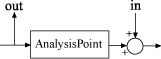
L is the open-loop transfer function from
in to out.
sign — Sign of transfer function for analysis
+1 (default) | -1
Sign of open-loop transfer function for analysis, specified as
+1 or -1.
By default, for an input closed-loop system T, the
function returns a transfer function L at the specified
analysis point, such that T = feedback(L,1,+1). However,
certain analysis commands that take an open-loop response assume that the
loop will be closed with negative feedback. For instance,
margin(L) computes the stability margin of the
negative feedback closed-loop system feedback(L,1).
Similarly, the stability margins you can obtain by right-clicking on a
bode plot make the same assumption. Therefore, when
you use getLoopTransfer to extract an open-loop
transfer function with the purpose of analyzing closed-loop stability, you
can set sign = -1 to extract a
transfer function L such that T =
feedback(L,1).
For example, consider the following system, where T
is the closed-loop transfer function from r to
y.
![]()
By default, L = getLoopTransfer(T,'X') computes the
transfer function L =
–C(s)G(s),
such that T = feedback(L,1,+1). To compute the stability
margins at X using the margin
command, which assumes negative feedback, you must compute a transfer
function L =
C(s)G(s),
such that T = feedback(L,1). To do so, use L =
getLoopTransfer(T,'X',-1).
openings — Additional locations for opening feedback loops
character vector | cell array of character vectors
Additional locations for opening feedback loops for computation of the
open-loop response, specified as character vector or cell array of character
vectors that identify analysis-point locations in T.
Analysis-point locations are marked by AnalysisPoint
blocks in T. Any channel name contained in the
Location property of an
AnalysisPoint block in T is a
valid entry for openings.
Use openings when you want to compute the open-loop
response at one analysis-point location with other loops also open at other
locations. For example, in a cascaded loop configuration, you can calculate
the inner loop open-loop response with the outer loop also open. Use
getPoints(T) to get a full list of available
analysis-point locations in T.
Output Arguments
Tips
You can use
getLoopTransferto extract open-loop responses given a generalized model of the overall control system. This is useful, for example, for validating open-loop responses of a control system that you tune with the a tuning command such assystune.getLoopTransferis thegenssequivalent to the Simulink® Control Design™ commandgetLoopTransfer(Simulink Control Design), which works with theslTunerandslLinearizerinterfaces. Use the Simulink Control Design command when your control system is modeled in Simulink.
Version History
Introduced in R2012b
See Also
AnalysisPoint | getPoints | genss | getIOTransfer | systune | getLoopTransfer (Simulink Control Design)
You can also select a web site from the following list:
Americas
- América Latina (Español)
- Canada (English)
- United States (English)
Europe
- Belgium (English)
- Denmark (English)
- Deutschland (Deutsch)
- España (Español)
- Finland (English)
- France (Français)
- Ireland (English)
- Italia (Italiano)
- Luxembourg (English)
- Netherlands (English)
- Norway (English)
- Österreich (Deutsch)
- Portugal (English)
- Sweden (English)
- Switzerland
- United Kingdom (English)