AnalysisPoint
Points of interest for linear analysis
Description
AnalysisPoint is a Control Design Block for marking a location
in a control system model as a point of interest for linear analysis and controller tuning.
You can combine an AnalysisPoint block with numeric LTI models, tunable LTI
models, and other Control Design Blocks to build tunable models of control systems.
AnalysisPoint locations are available for analysis with commands such as
getIOTransfer or getLoopTransfer. Such locations
are also available for specifying design goals for control system tuning.
You can combine an AnalysisPoint block with numeric LTI models, tunable
LTI models, and other Control Design Blocks to build tunable models of control systems.
AnalysisPoint locations are available for analysis with commands such as
getIOTransfer or getLoopTransfer. Such locations
are also available for specifying design goals for control system tuning.
For example, consider the following control system.

Suppose that you are interested in the effects of disturbance injected at
u in this control system. Inserting an AnalysisPoint
block at the location u associates an implied input, implied output, and
the option to open the loop at that location, as in the following diagram.

Suppose that T is a model of the control system including the
AnalysisPoint block, AP_u. In this case, the command
getIOTransfer(T,'AP_u','y') returns a model of the closed-loop transfer
function from u to y. Likewise, the command
getLoopTransfer(T,'AP_u',-1) returns a model of the negative-feedback
open-loop response, CG, measured at the location u.
AnalysisPoint blocks are also useful when tuning a control system
using tuning commands such as systune. You can use an
AnalysisPoint block to mark a loop-opening location for open-loop
tuning requirements such as TuningGoal.LoopShape or
TuningGoal.Margins. You can also use an AnalysisPoint
block to mark the specified input or output for tuning requirements such as
TuningGoal.Gain. For example, Req =
TuningGoal.Margins('AP_u',5,40) constrains the gain and phase margins at the
location u.
You can create AnalysisPoint blocks explicitly using the
AnalysisPoint command and connect them with other block diagram
components using model interconnection commands. For example, the following code creates a
model of the system illustrated above.
G = tf(1,[1 2]);
C = tunablePID('C','pi');
AP_u = AnalysisPoint('u');
T = feedback(G*AP_u*C,1);      % closed loop r->y
You can also create analysis points implicitly, using the connect
command. The following syntax creates a dynamic system model with analysis points, by
interconnecting multiple models sys1,sys2,...,sysN:
sys = connect(sys1,sys2,...,sysN,inputs,outputs,APs);
APs lists the signal locations at which to insert analysis points. The
software automatically creates and inserts an AnalysisPoint block with
channels corresponding to these locations. See connect for more information.
Creation
Description
AP = AnalysisPoint(name)AP anywhere in the
generalized model of your control system to mark a point of interest for linear analysis
or controller tuning. name specifies the block name.
Input Arguments
Properties
Location — Names of channels in the AnalysisPoint blocks
'AP' (default) | character vector
Names of channels in the AnalysisPoint blocks, specified as a
character vector or a cell array of character vectors.
By default, the analysis-point channels are named after the
name argument. For example, if you have a single-channel analysis
point, AP, that has name 'AP', then
AP.Location = 'AP' by default. If you have a multi-channel analysis
point, then AP.Location = {'AP(1)','AP(2)',...} by default. Set
AP.Location to a different value if you want to customize the
channel names.
Data Types: char | cell
Open — Loop-opening state
0 (default) | 1
Loop-opening state, specified as a logical value or vector of logical values. This property tracks whether the loop is open or closed at the analysis point.
For example, consider the feedback loop of the following illustration.
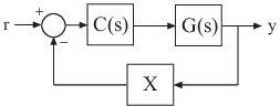
You can model this feedback loop as follows.
G = tf(1,[1 2]);
C = tunablePID('C','pi');
X = AnalysisPoint('X');
T = feedback(G*C,X);
T.InputName = 'r';
T.OutputName = 'y';
By default, the analysis point at X is closed. You can get the
transfer function from r to y with the feedback
loop open at X as follows.
Try = getIOTransfer(T,'r','y','X');
In the resulting generalized state-space (genss) model, the
AnalysisPoint block 'X' is marked open. In
other words, Try.Blocks.X.Open = 1.
For a multi-channel analysis point, then Open is a logical vector
with as many entries as the analysis point has channels.
Data Types: logical
Ts — Sample time
0 (continuous time) (default)
Sample time. For AnalysisPoint blocks, the value of this
property is automatically set to the sample time of other blocks and models you connect
it with.
Data Types: double
Examples
Feedback Loop with Analysis Point
Create a model of the following feedback loop with an analysis point in the feedback path.

For this example, the plant model is . C is a tunable PI controller, and X is the analysis point.
G = tf(1,[1 2]);
C = tunablePID('C','pi');
X = AnalysisPoint('X');
T = feedback(G*C,X);
T.InputName = 'r';
T.OutputName = 'y';
T is a tunable genss model. T.Blocks contains the Control Design Blocks of the model, which are the controller, C, and the analysis point, X.
T.Blocks
ans = struct with fields:
    C: [1x1 tunablePID]
    X: [1x1 AnalysisPoint]
Examine the step response of T.
stepplot(T)

The presence of the AnalysisPoint block does not change the dynamics of the model.
You can use the analysis point for linear analysis of the system. For instance, extract the system response at 'y' to a disturbance injected at the analysis point.
Txy = getIOTransfer(T,'X','y');
The AnalysisPoint block also allows you to temporarily open the feedback loop at that point. For example, compute the open-loop response from 'r' to 'y'.
Try_open = getIOTransfer(T,'r','y','X');
Specifying the analysis point name as the last argument to getIOTransfer extracts the response with the loop open at that point. Examine the step response of Try_open to verify that it is the open-loop response.
stepplot(Try_open);

Feedback Loop with Analysis Point
Consider the following block diagram.

You can create a model of this closed-loop system using feedback and use the model to study the system response from r to y. Suppose that you also want to study the response of the closed-loop system to a disturbance injected at the plant input. To do so, you can use connect to build the system, inserting an analysis point at the location u.
First create plant and controller models, naming the inputs and outputs as shown in the diagram.
C = pid(2,1);
C.InputName = "e";
C.OutputName = "u";

G = zpk([],[-1,-1],1);
G.InputName = "u";
G.OutputName = "y";
Create a summing junction that takes the difference between the reference signal r and the plant output y to compute the error signal e.
Sum = sumblk("e = r - y");Combine C, G, and the summing junction to create the aggregate model. Use the APs input argument to connect to insert an analysis point at u.
input = "r";
output = "y";
APs = "u";
CL = connect(G,C,Sum,input,output,APs)
Generalized continuous-time state-space model with 1 outputs, 1 inputs, 3 states, and the following blocks:
  CONNECT_AP1: Analysis point, 1 channels, 1 occurrences.

Type "ss(CL)" to see the current value and "CL.Blocks" to interact with the blocks.
This closed-loop model is a generalized state-space (genss) model containing an AnalysisPoint control design block. To see the name of the analysis point channel in CL, use getPoints.
getPoints(CL)
ans = 1x1 cell array
    {'u'}
Inserting the analysis point creates a model that is equivalent to the following block diagram, where AP_u designates the AnalysisPoint block with channel name u.

Use the analysis point to extract system responses. For example, the following commands extract the open-loop transfer at u and the closed-loop response at y to a disturbance injected at u.
L = getLoopTransfer(CL,"u",-1);
CLdist = getIOTransfer(CL,"u","y");
Multi-Channel Analysis Points
Create a block for marking two analysis points in a MIMO model.
In the control system of the following illustration, consider each signal a vector-valued signal of size 2. In other words, the signal represents {r(1),r(2)}, represents {y(1),y(2)}, and so on.

The feedback signal is therefore also a vector-valued signal of size 2. Create a block for marking the two analysis points in the feedback path.
AP = AnalysisPoint('X',2)Multi-channel analysis point at locations: X(1) X(2) Type "ss(AP)" to see the current value.
The AnalysisPoint block is stored as a variable in the MATLAB® workspace called AP. In addition, the Name property of the block is set to X. When you interconnect the block with numeric LTI models or other Control Design Blocks, this analysis-point block is identified in the Blocks property of the resulting genss model as X. The block name X is automatically expanded to generate the channel names X(1) and X(2).
It is sometimes convenient to change the channel names to match the names of the signals they correspond to in a block diagram of your model. For example, suppose the points of interest you want to mark in your model are signals named L and V. Change the Location property of AP to make the names match those signals.
AP.Location = {'L';'V'}Multi-channel analysis point at locations: L V Type "ss(AP)" to see the current value.
Although the channel names have changed, the block name remains X.
AP.Name
ans =
'X'
Therefore, the Blocks property of a genss model you build with this block still identifies the block as X. Use getPoints to find the channel names of available analysis points in a genss model.
Version History
Introduced in R2014b
You can also select a web site from the following list:
Americas
- América Latina (Español)
- Canada (English)
- United States (English)
Europe
- Belgium (English)
- Denmark (English)
- Deutschland (Deutsch)
- España (Español)
- Finland (English)
- France (Français)
- Ireland (English)
- Italia (Italiano)
- Luxembourg (English)
- Netherlands (English)
- Norway (English)
- Österreich (Deutsch)
- Portugal (English)
- Sweden (English)
- Switzerland
- United Kingdom (English)