Compare Reference Signal Overhead with Channel Estimation Accuracy for 6G

Since R2026a

This example shows how to use custom reference signals (RSs) to explore the tradeoff between RS overhead and channel estimation accuracy.

Introduction

6G Exploration Library for 5G Toolbox™ enables you to design custom reference signals without the limitations of 5G. Reference signal design involves a fundamental tradeoff: denser RS patterns improve channel estimation accuracy but use resource elements that could otherwise carry data. For 6G systems with wide bandwidths and high subcarrier spacings, this tradeoff becomes critical because the coherence bandwidth and time may be shorter, requiring more pilots. This example explores different RS densities and measures their effect on channel estimation accuracy

Configure Carrier

Create a carrier with 120 kHz subcarrier spacing and 275 resource blocks. This corresponds to an available bandwidth of 396 MHz.

carrier = pre6GCarrierConfig(SubcarrierSpacing=120,NSizeGrid=275);
ofdmInfo = pre6GOFDMInfo(carrier);
disp(['Transmission bandwidth = ' num2str(carrier.NSizeGrid*12*carrier.SubcarrierSpacing*1e3/1e6) ' MHz'])

Transmission bandwidth = 396 MHz

Create a set of RS configurations with four different RS densities. Each configuration places RS on a different number of subcarrier locations per physical resource block (PRB).

• Light: One subcarrier per PRB, one symbol

• Medium: Two subcarriers per PRB, two symbols

• Heavy: Four subcarriers per PRB, four symbols

• Ultra-dense: Six subcarriers per PRB, four symbols

rsConfigs = cell(1,4);
labels = ["Light" "Medium" "Heavy" "Ultra-Dense"];

rsConfigs{1} = pre6GReferenceSignalConfig;
rsConfigs{1}.PRBSet = 0:carrier.NSizeGrid-1;
rsConfigs{1}.SubcarrierLocations = 0;
rsConfigs{1}.SymbolLocations = 0;

rsConfigs{2} = pre6GReferenceSignalConfig;
rsConfigs{2}.PRBSet = 0:carrier.NSizeGrid-1;
rsConfigs{2}.SubcarrierLocations = [0;6];
rsConfigs{2}.SymbolLocations = [0;7];

rsConfigs{3} = pre6GReferenceSignalConfig;
rsConfigs{3}.PRBSet = 0:carrier.NSizeGrid-1;
rsConfigs{3}.SubcarrierLocations = [0;3;6;9];
rsConfigs{3}.SymbolLocations = [0;4;7;11];

rsConfigs{4} = pre6GReferenceSignalConfig;
rsConfigs{4}.PRBSet = 0:carrier.NSizeGrid-1;
rsConfigs{4}.SubcarrierLocations = [0;2;4;6;8;10];
rsConfigs{4}.SymbolLocations = [0;4;7;11];

Calculate RS Overhead

For each configuration, calculate the number of RS resource elements and the resulting overhead as a fraction of the total grid.

totalREs = carrier.NSizeGrid * 12 * carrier.SymbolsPerSlot;
overhead = zeros(1,4);
numRSREs = zeros(1,4);
rsInd = cell(1,4);

for i = 1:4
      rsInd{i} = pre6GReferenceSignalIndices(carrier,rsConfigs{i});
      numRSREs(i) = numel(rsInd{i});
      overhead(i) = numRSREs(i) / totalREs * 100;
end

Display the overhead for each configuration.

for i = 1:4
      disp([char(labels(i)) ': ' num2str(numRSREs(i)) ' REs (' num2str(overhead(i),'%.1f') '% overhead)'])
end

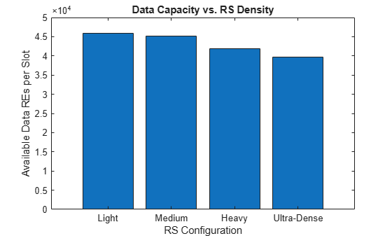
Light: 275 REs (0.6% overhead)
Medium: 1100 REs (2.4% overhead)
Heavy: 4400 REs (9.5% overhead)
Ultra-Dense: 6600 REs (14.3% overhead)

Show the remaining capacity for data symbols after RS allocation.

figure;
bar(categorical(labels,labels),totalREs - numRSREs);
xlabel('RS Configuration');
ylabel('Available Data REs per Slot');
title('Data Capacity vs. RS Density');

Simulate Channel Estimation With AWGN

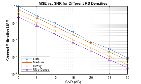
For each RS configuration, transmit through an AWGN channel at varying signal-to-noise ratio (SNR) levels and measure the channel estimation mean squared error.

snrRange = 0:5:30;
mseResults = zeros(4,numel(snrRange));
numTxAnts =1;

for i = 1:4
      txGrid = pre6GResourceGrid(carrier,numTxAnts);
      rsInd = pre6GReferenceSignalIndices(carrier,rsConfigs{i});
      rsSym = pre6GReferenceSignal(carrier,rsConfigs{i});
      txGrid(rsInd) = rsSym;

      for s = 1:numel(snrRange)
          rxGrid = awgn(txGrid,snrRange(s));
          [H,~] = pre6GChannelEstimate(carrier,rsConfigs{i},rxGrid);
          rsEst = H(rsInd);
          mseResults(i,s) = mean(abs(rsEst - 1).^2);
      end
end

Plot MSE for RS Configurations

Plot the MSE as a function of SNR for all RS densities.

  figure;
  semilogy(snrRange,mseResults(1,:),'-o',snrRange,mseResults(2,:),'-s', ...
      snrRange,mseResults(3,:),'-d',snrRange,mseResults(4,:),'-^');
  xlabel('SNR (dB)');
  ylabel('Channel Estimation MSE');
  title('MSE vs. SNR for Different RS Densities');
  legend(labels,Location='southwest');
  grid on;