Model Engine Timing Using Triggered Subsystems
This example shows how to model a four-cylinder spark ignition internal combustion engine from the throttle to the crankshaft output using triggered subsystems. In this example, the sldemo_engine model is based on [1].
The sldemo_engine model uses the Triggered Subsystem blocks in the Valve Timing and Combustion subsystems. In this example, the tasks of all four cylinders are implemented with one set of blocks instead of four sets of blocks, one set per cylinder.
Open the model.
open_system('sldemo_engine')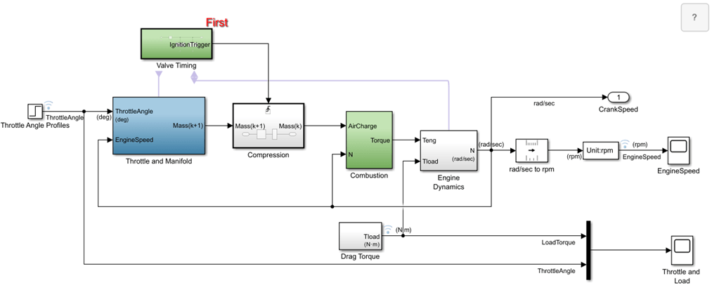
In an inline four-cylinder four-stroke engine, 180 degrees of crankshaft rotation separates the ignition of each successive cylinder. This separation means that each cylinder fires on every other crank revolution. In this model, the intake, compression, combustion, and exhaust strokes occur simultaneously (at any given time, one cylinder is in each phase). To account for compression, the combustion of each intake charge is delayed by 180 degrees of crank rotation from the end of the intake stroke.
In this model, an Integrator block accumulates the cylinder mass air flow in the Intake Manifold block located inside the Throttle and Manifold subsystem. The Valve Timing subsystem generates pulses that correspond to specific rotational positions to manage the crank angle, air-fuel mass and triggers execution of Compression subsystem. The Compression subsystem uses a Unit Delay block to insert 180 degree (one event period) of delay between the intake and combustion of each air-fuel charge.
Consider a complete four-stroke cycle for one cylinder. The following describes the functionality of each stroke.
Intake stroke During this stroke, the intake manifold opens and takes in the air-fuel mixture. The piston moves from the top dead center (TDC) to the bottom dead center (BDC) and the crank shaft completes 180 degrees rotation. In this model, the
Intake Manifoldsubsystem inside theThrottle and Manifoldsubsystem integrates the mass flow rate from the manifold.Compression stroke During this stroke, the intake manifold closes and the air-fuel charge is compressed by 180 degrees rotation of the crank shaft. The piston moves from BDC to TDC. Due to compression, the temperature of the air-fuel mixture increases which assists the combustion process.
Combustion stroke The spark plug ignites the air-fuel mixture. Combustion of the mixture inside the cylinder generates pressure that forces the piston to move from TDC to BDC. During this stroke, the crank shaft rotates by 180 degrees and generates torque.
Exhaust stroke During the exhaust stroke, the piston moves from BDC to TDC by 180 degrees rotation of the crank shaft. When the piston head reaches TDC, the exhaust manifold opens and let the exhaust out of the cylinder. In this model, the Integrator block inside the
Throttle and Manifoldsubsystem is reset and prepared for the next cycle of four strokes (720 degrees) of this cylinder.
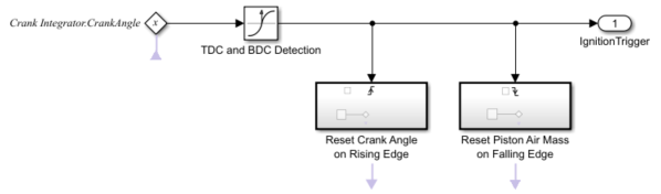
Valve Timing
The Valve Timing subsystem controls valve timing (opening and closing), triggers ignition, and resets the crank shaft angle based on the angular position of the engine crank shaft. The Valve Timing subsystem contains two Triggered subsystem blocks: Reset Crank Angle on Rising Edge and Reset Piston Air Mass on Falling Edge.
Reset Piston Air Mass on Falling Edge is triggered when the crankshaft moves from TDC to BDC, and transfers the air-fuel mixture from the intake manifold to the cylinders via discrete valve events. The transfer process takes place concurrently with the continuous-time processes of intake flow, torque generation, and acceleration.
Reset Crank Angle on Rising Edge is triggered once the crankshaft angle exceeds 180 degrees, and resets the angle to 0 degrees.
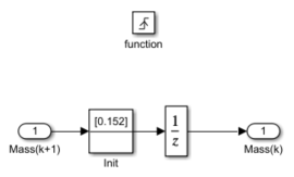
Compression
The Compression subsystem represents the engine dynamics during the compression stroke. This subsystem is triggered when it receives a positive trigger value at the Trigger port of the block. The Unit Delay block samples the integrator state. This value, the accumulated mass charge, is available at the output of the Compression subsystem for use during combustion.
Throttle and Manifold
The throttle body of the engine is modeled by the Throttle and Manifold subsystem.
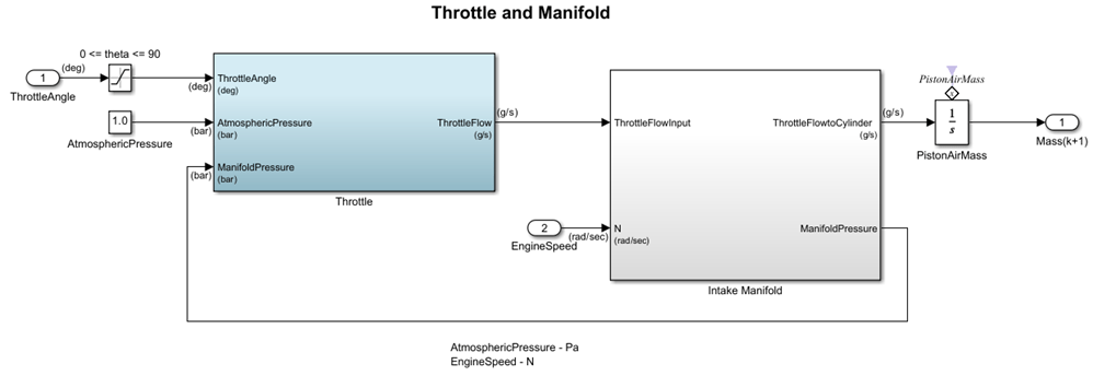
Throttle
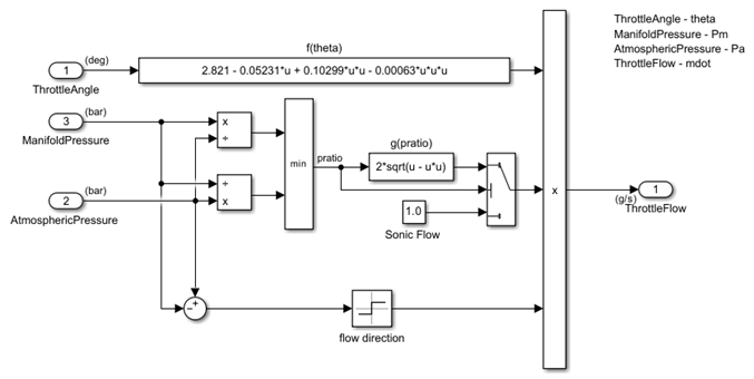
The Throttle subsystem uses throttle plate angle (), manifold pressure (), and atmospheric pressure () as inputs. The air-fuel mixture intake rate() at the intake manifold can be expressed as the product of two functions:
Empirical function of the throttle plate angle
Function of the atmospheric and manifold pressures
In cases of lower manifold pressure (greater vacuum), the flow rate through the throttle body is sonic and is only a function of the throttle angle. This model accounts for this low pressure behavior with a switching condition in the following compressibility equations.
Equation 1
The individual equations, mentioned above, are incorporated using Fcn blocks. A Switch block determines whether the flow is sonic by comparing the pressure ratio to its switch threshold. In the sonic regime, the flow rate is a function of the throttle position only. The direction of flow is from the higher to lower pressure, as determined by the Sign block. The MinMax block ensures that the pressure ratio is always unity or less.
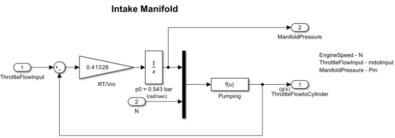
Intake Manifold
The Throttle and Manifold subsystem contains the Intake Manifold subsystem. This subsystem uses the throttle flow input and engine speed () as inputs. The intake manifold is modeled as a differential equation for the manifold pressure (). The difference in the incoming and outgoing mass flow rates represents the net rate of change of air mass with respect to time. This quantity, according to the ideal gas law, is proportional to the time derivative of the manifold pressure.
However, unlike the model in [1], this model does not incorporate exhaust gas recirculation (EGR).
Equation 2
The mass flow rate of air-fuel mixture that the model pumps into the cylinders from the manifold is described in the following empirical equation. This mass rate () is a function of the manifold pressure () and the engine speed ().
Equation 3
To determine the total air-fuel mixture charge pumped into the cylinders, the simulation integrates the mass flow rate from the intake manifold and samples it at the end of each intake stroke event. This sampling determines the total air mass that is present in each cylinder after the intake stroke and before compression.
The Intake Manifold subsystem is used to model the throttle dynamics expressed in Equation 2. The differential equation from Equation 2 models the intake manifold pressure. A Simulink Function block computes the mass flow rate into the cylinder, a function of manifold pressure and engine speed, expressed in Equation 3.
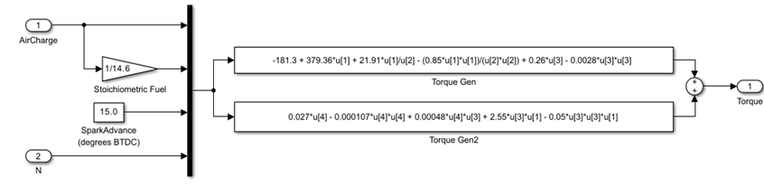
Combustion
Torque is generated during the combustion stroke. The Combustion subsystem models the combustion process and torque generation using four variables, expressed in Equation 4. The model uses a Mux block to combine these variables into a vector that provides input to the Fcn block that incorporates the equation.
Equation 4
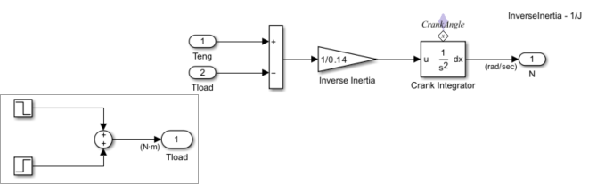
Engine Dynamics
The Engine Dynamics subsystem computes the engine speed () and crank angle using the load torque and the generated torque . is computed using step functions in the Drag Torque subsystem. Engine speed is computed using the equation , where J is the engine rotational moment of inertia .
Simulate the Model and Visualize the Results
Simulate the model and visualize the results using plot function.
sim('sldemo_engine'); The default input values are used for simulation:
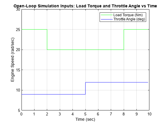
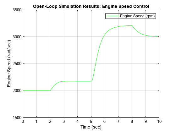
Simulink® returns the simulated engine speed, the throttle commands that drive the simulation, and the load torque that disturbs it.
The model logs this data to the base workspace in a structure, sldemo_engine_output.
PlotHandle = plot(sldemo_engine_output.get('LoadTorque').Values.Time, ...
               sldemo_engine_output.get('LoadTorque').Values.Data, 'g', ...
               sldemo_engine_output.get('ThrottleAngle').Values.Time, ...
               sldemo_engine_output.get('ThrottleAngle').Values.Data, 'b'  );
title('Open-Loop Simulation Inputs: Load Torque and Throttle Angle vs Time');
xlabel('Time (sec)'); ylabel('Engine Speed (rad/sec)');
set(gca,'Color','w','XGrid','On','XColor',[0 0 0],...
                    'YGrid','On','YColor',[0 0 0]);
axis([0 10 5 30]);
h= legend('Load Torque (Nm)','Throttle Angle (deg)','Location','northeast');
set(h,'TextColor','k','Color','none');
PlotHandle = plot(sldemo_engine_output.get('EngineSpeed').Values.Time, ...
                  sldemo_engine_output.get('EngineSpeed').Values.Data,'g'  );
title('Open-Loop Simulation Results: Engine Speed Control');
xlabel('Time (sec)'); ylabel('Engine Speed (rad/sec)');
set(gca,'Color','w','XGrid','On','XColor',[0 0 0],...
                    'YGrid','On','YColor',[0 0 0]);
axis([0 10 1500 3500]);
h = legend('Engine Speed (rpm)','Location','northeast');
set(h,'TextColor','k','Color','none');
See Also
Triggered Subsystem | State Writer | State Reader | Integrator | Second-Order Integrator | Mux | Step
Related Topics
- Enable Signal Logging for Model
- Engine Timing Model with Closed Loop Control
- Powertrain Blockset
- Specify Block Execution Order, Execution Priority and Tag
References
[1] Crossley, P. R., and J. A. Cook. “A Nonlinear Engine Model for Drivetrain System Development.” International Conference on Control 1991. Control ’91 1991, pp. 921–25 vol.2. IEEE Xplore, DOI.org (Crossref), https://ieeexplore.ieee.org/abstract/document/98573.
[2] The Simulink Model. Developed by Ken Butts, Ford Motor Company. Modified by Paul Barnard, Ted Liefeld and Stan Quinn, MathWorks®, 1994 — 7."
[3] Moskwa, John J., and J. Karl Hedrick. “Automotive Engine Modeling for Real Time Control Application.” 1987 American Control Conference, 1987, pp. 341–46. IEEE Xplore, DOIː 10.23919/ACC.1987.4789343.
[4] Powell, B. K., and J. A. Cook. “Nonlinear Low Frequency Phenomenological Engine Modeling and Analysis.” 1987 American control conference, 1987, pp. 332–40. IEEE Xplore, DOIː 10.23919/ACC.1987.4789342.
[5] Weeks, Robert W., and John J. Moskwa. “Automotive Engine Modeling for Real-Time Control Using MATLAB/SIMULINK.” SAE transactions, vol. 104, 1995, pp. 295–309. JSTOR, https://www.jstor.org/stable/44473229.
You can also select a web site from the following list:
Americas
- América Latina (Español)
- Canada (English)
- United States (English)
Europe
- Belgium (English)
- Denmark (English)
- Deutschland (Deutsch)
- España (Español)
- Finland (English)
- France (Français)
- Ireland (English)
- Italia (Italiano)
- Luxembourg (English)
- Netherlands (English)
- Norway (English)
- Österreich (Deutsch)
- Portugal (English)
- Sweden (English)
- Switzerland
- United Kingdom (English)