Spectral Analysis of Nonuniformly Sampled Signals
This example shows how to perform spectral analysis on nonuniformly sampled signals. It helps you determine if a signal is uniformly sampled or not, and if not, it shows how to compute its spectrum or its power spectral density.
The example introduces the Lomb-Scargle periodogram, which can compute spectra of nonuniformly sampled signals.
Nonuniformly Sampled Signals
Nonuniformly sampled signals are often found in the automotive industry, in communications, and in fields as diverse as medicine and astronomy. Nonuniform sampling might be due to imperfect sensors, mismatched clocks, or event-triggered phenomena.
The computation and study of spectral content is an important part of signal analysis. Conventional spectral analysis techniques like the periodogram and the Welch method require the input signal to be uniformly sampled. When the sampling is nonuniform, one can resample or interpolate the signal onto a uniform sample grid. This, however, can add undesired artifacts to the spectrum and might lead to analysis errors.
A better alternative is to use the Lomb-Scargle method, which works directly with the nonuniform samples and thus makes it unnecessary to resample or interpolate. The algorithm has been implemented in the plomb function.
Spectral Analysis of Signals with Missing Data
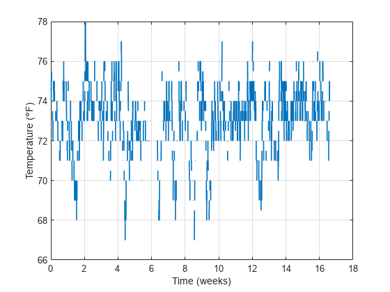
Consider a temperature monitoring system in which a microcontroller records the temperature of a room and transmits this reading every 15 minutes to a cloud-based server that stores it. It is known that glitches in internet connectivity prevent the cloud-based system from receiving some of the readings sent by the microcontroller. Also, at least once during the measurement period the microcontroller's battery ran out, leading to a large gap in the sampling.
Load the temperature readings and the corresponding timestamps.
load('nonuniformdata.mat','roomtemp','t1')

figure
plot(t1/(60*60*24*7),roomtemp,'LineWidth',1.2)

grid
xlabel('Time (weeks)')
ylabel('Temperature (\circF)')
An easy way to determine if a signal is uniformly sampled is to take a histogram of the intervals between successive sample times.
Plot a histogram of sampling intervals (time differences) in minutes. Include only points at which samples are present.
tAtPoints = t1(~isnan(roomtemp))/60;
TimeIntervalDiff = diff(tAtPoints);

figure
hist(TimeIntervalDiff,0:100)
grid
xlabel('Sampling intervals (minutes)')
ylabel('Occurrences')
xlim([10 100])
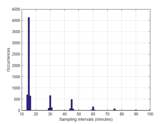
The majority of the measurements are spaced approximately 15 minutes apart, as expected. However, a fair number of occurrences have sampling intervals of around 30 and 45 minutes, which correspond to one or two consecutive dropped samples. This causes the signal to be nonuniformly sampled. Furthermore, the histogram shows some jitter surrounding the bars showing high occurrences. This could relate to TCP/IP latency.
Use the Lomb-Scargle method to compute and visualize the spectral content of the signal. To help visualize the spectrum better, consider frequencies up to 0.02 mHz, which correspond to about 13 cycles per week.
[Plomb,flomb] = plomb(roomtemp,t1,2e-5,'power');

figure
plot(flomb*60*60*24*7,Plomb)
grid
xlabel('Frequency (cycles/week)')
ylabel('Power (dBW)')
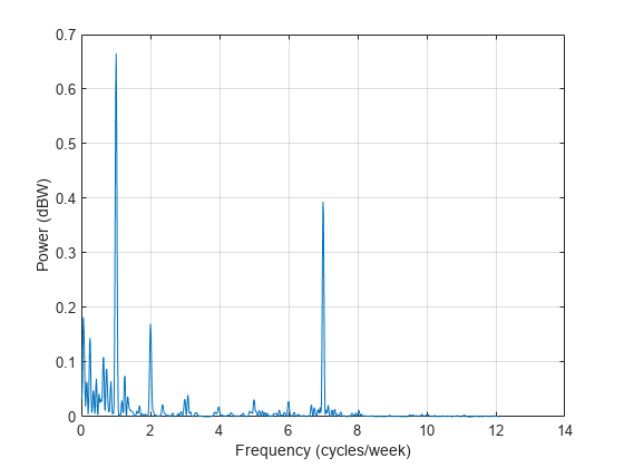
The spectrum shows dominant periodicities at 7 cycles per week and 1 cycle per week. This is understandable, given that the data comes from a temperature-controlled building on a seven-day calendar. The spectral line showing a peak at 1 cycle per week indicates that the temperature in the building follows a weekly cycle, with lower temperatures on weekends and higher temperatures during the week. The spectral line of 7 cycles per week indicates that there is also a daily cycle with lower temperatures at night and higher temperatures during the day.
Spectral Analysis of Signals with Unevenly Spaced Samples
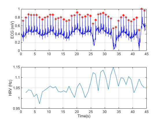
Heart-rate variability (HRV) signals, which represent the physiological variation in time between heartbeats, are typically unevenly sampled because human heart rates are not constant. HRV signals are derived from electrocardiogram (ECG) readings.
The sample points of an HRV signal are located at the R-Peak times of the ECG. The amplitude of each point is computed as the inverse of the time difference between consecutive R-Peaks and is placed at the instant of the second R-Peak.
% Load the signal, the timestamps, and the sample rate
load('nonuniformdata.mat','ecgsig','t2','Fs')

% Find the ECG peaks
[pks,locs] = findpeaks(ecgsig,Fs, ...
    'MinPeakProminence',0.3,'MinPeakHeight',0.2);

% Determine the RR intervals
RLocsInterval = diff(locs);

% Derive the HRV signal
tHRV = locs(2:end);
HRV = 1./RLocsInterval;

% Plot the signals
figure
a1 = subplot(2,1,1);
plot(t2,ecgsig,'b',locs,pks,'*r')
grid
a2 = subplot(2,1,2);
plot(tHRV,HRV)
grid
xlabel(a2,'Time(s)')
ylabel(a1,'ECG (mV)')
ylabel(a2,'HRV (Hz)')
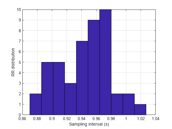
The varying intervals between the R-peaks cause the sample-time nonuniformity in the HRV data. Consider the peak locations of the signal and plot a histogram of their separations in seconds.
figure
hist(RLocsInterval)

grid
xlabel('Sampling interval (s)')
ylabel('RR distribution')
The typical frequency bands of interest in HRV spectra are:
Very Low Frequency (VLF), from 3.3 to 40 mHz,
Low Frequency (LF), from 40 to 150 mHz,
High Frequency (HF), from 150 to 400 mHz.
These bands approximately confine the frequency ranges of the distinct biological regulatory mechanisms that contribute to HRV. Fluctuations in any of these bands have biological significance.
Use plomb to calculate the spectrum of the HRV signal.
figure
plomb(HRV,tHRV,'Pd',[0.95, 0.5])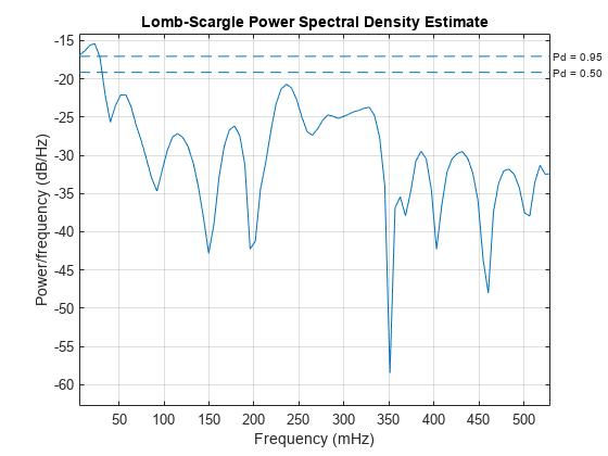
The dashed lines denote 95% and 50% detection probabilities. These thresholds measure the statistical significance of peaks. The spectrum shows peaks in all three bands of interest listed above. However, only the peak located at 23.2 mHz in the VLF range shows a detection probability 95%, while the other peaks have detection probabilities of less than 50%. The peaks lying below 40 mHz are thought to be due to long-term regulatory mechanisms, such as the thermoregulatory system and hormonal factors.