plot3
3-D line plot
Syntax
Description
Vector and Matrix Data
plot3(
assigns specific line styles, markers, and colors to each X1,Y1,Z1,LineSpec1,...,Xn,Yn,Zn,LineSpecn)XYZ triplet.
You can specify LineSpec for some triplets and omit it for others. For
example, plot3(X1,Y1,Z1,'o',X2,Y2,Z2) specifies markers for the first
triplet but not for the second triplet.
Table Data
plot3(
plots the variables tbl,xvar,yvar,zvar)xvar, yvar, and
zvar from the table tbl. To plot one data set,
specify one variable each for xvar, yvar, and
zvar. To plot multiple data sets, specify multiple variables for at
least one of those arguments. The arguments that specify multiple variables must specify
the same number of variables. (since R2022a)
Additional Options
plot3( displays the plot
in the target axes. Specify the axes as the first argument in any of the previous
syntaxes.ax,___)
plot3(___, specifies
Name,Value)Line properties using one or more name-value pair arguments. Specify
the properties after all other input arguments. For a list of properties, see Line Properties.
p = plot3(___)Line object or an array of Line objects. Use
p to modify properties of the plot after creating it. For a list of
properties, see Line Properties.
Examples
Plot 3-D Helix
Define t as a vector of values between 0 and 10. Define st and ct as vectors of sine and cosine values. Then plot st, ct, and t.
t = 0:pi/50:10*pi;
st = sin(t);
ct = cos(t);
plot3(st,ct,t)

Plot Multiple Lines
Create two sets of x-, y-, and z-coordinates.
t = 0:pi/500:pi;
xt1 = sin(t).*cos(10*t);
yt1 = sin(t).*sin(10*t);
zt1 = cos(t);

xt2 = sin(t).*cos(12*t);
yt2 = sin(t).*sin(12*t);
zt2 = cos(t);
Call the plot3 function, and specify consecutive XYZ triplets.
plot3(xt1,yt1,zt1,xt2,yt2,zt2)
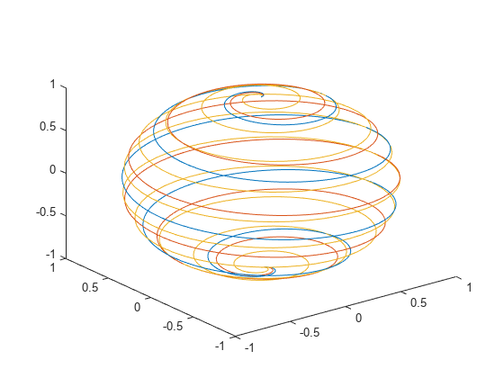
Plot Multiple Lines Using Matrices
Create matrix X containing three rows of x-coordinates. Create matrix Y containing three rows of y-coordinates.
t = 0:pi/500:pi;
X(1,:) = sin(t).*cos(10*t);
X(2,:) = sin(t).*cos(12*t);
X(3,:) = sin(t).*cos(20*t);

Y(1,:) = sin(t).*sin(10*t);
Y(2,:) = sin(t).*sin(12*t);
Y(3,:) = sin(t).*sin(20*t);
Create matrix Z containing the z-coordinates for all three sets.
Z = cos(t);
Plot all three sets of coordinates on the same set of axes.
plot3(X,Y,Z)
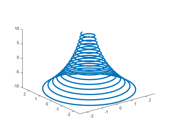
Specify Equally-Spaced Tick Units and Axis Labels
Create vectors xt, yt, and zt.
t = 0:pi/500:40*pi;
xt = (3 + cos(sqrt(32)*t)).*cos(t);
yt = sin(sqrt(32) * t);
zt = (3 + cos(sqrt(32)*t)).*sin(t);
Plot the data, and use the axis equal command to space the tick units equally along each axis. Then specify the labels for each axis.
plot3(xt,yt,zt)
axis equal
xlabel('x(t)')
ylabel('y(t)')
zlabel('z(t)')

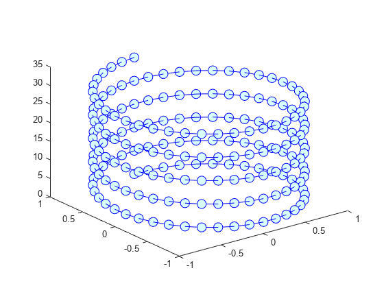
Plot Points as Markers Without Lines
Create vectors t, xt, and yt, and plot the points in those vectors using circular markers.
t = 0:pi/20:10*pi;
xt = sin(t);
yt = cos(t);
plot3(xt,yt,t,'o')
Customize Color and Marker
Create vectors t, xt, and yt, and plot the points in those vectors as a blue line with 10-point circular markers. Use a hexadecimal color code to specify a light blue fill color for the markers.
t = 0:pi/20:10*pi;
xt = sin(t);
yt = cos(t);
plot3(xt,yt,t,'-o','Color','b','MarkerSize',10,...
    'MarkerFaceColor','#D9FFFF')
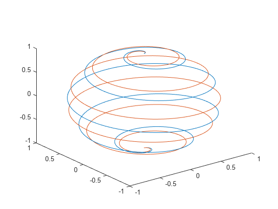
Specify Line Style
Create vector t. Then use t to calculate two sets of x and y values.
t = 0:pi/20:10*pi;
xt1 = sin(t);
yt1 = cos(t);

xt2 = sin(2*t);
yt2 = cos(2*t);
Plot the two sets of values. Use the default line for the first set, and specify a dashed line for the second set.
plot3(xt1,yt1,t,xt2,yt2,t,'--')
Modify Line After Plotting
Create vectors t, xt, and yt, and plot the data in those vectors. Return the chart line in the output variable p.
t = linspace(-10,10,1000);
xt = exp(-t./10).*sin(5*t);
yt = exp(-t./10).*cos(5*t);
p = plot3(xt,yt,t);
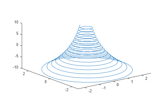
Change the line width to 3.
p.LineWidth = 3;
Plot Data from a Table
Since R2022a
A convenient way to plot data from a table is to pass the table to the plot3 function and specify the variables to plot.
Create vectors x, y, and t, and put the vectors in a table. Then display the first three rows of the table.
t = (0:pi/20:10*pi)';
x = sin(t);
y = cos(t);
tbl = table(x,y,t);
head(tbl,3)
       x          y          t
    _______    _______    _______

          0          1          0
    0.15643    0.98769    0.15708
    0.30902    0.95106    0.31416
Plot the x, y, and t table variables. Return the Line object as p. Notice that the axis labels match the variable names.
p = plot3(tbl,"x","y","t");

To modify aspects of the line, set the LineStyle, Color, and Marker properties on the Line object. For example, change the line to a red dotted line with circular markers.
p.LineStyle = ":";
p.Color = "red";
p.Marker = "o";

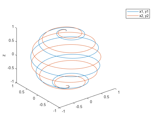
Plot Multiple Table Variables on the x- and y-Axes
Since R2022a
Create a table containing five variables. Then display the first three rows of the table.
t = (0:pi/500:pi)';
x1 = sin(t).*cos(10*t);
x2 = sin(t).*cos(12*t);
y1 = sin(t).*sin(10*t);
y2 = sin(t).*sin(12*t);
z = cos(t);
tbl = table(x1,x2,y1,y2,z);
head(tbl,3)
       x1           x2            y1            y2           z
    _________    _________    __________    __________    _______

            0            0             0             0          1
    0.0062707    0.0062653    0.00039452    0.00047329    0.99998
     0.012467     0.012423     0.0015749     0.0018877    0.99992
Plot the x1 and x2 variables on the x-axis, the y1 and y2 variables on the y-axis, and the z variable on the z-axis. Then add a legend. Notice that the legend entries match the variable names.
plot3(tbl,["x1","x2"],["y1","y2"],"z")
legend
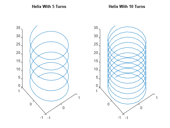
Specify Target Axes
Starting in R2019b, you can display a tiling of plots using the tiledlayout and nexttile functions. Call the tiledlayout function to create a 1-by-2 tiled chart layout. Call the nexttile function to create the axes objects ax1 and ax2. Create separate line plots in the axes by specifying the axes object as the first argument to plot3.
tiledlayout(1,2)

% Left plot
ax1 = nexttile;
t = 0:pi/20:10*pi;
xt1 = sin(t);
yt1 = cos(t);
plot3(ax1,xt1,yt1,t)
title(ax1,'Helix With 5 Turns')

% Right plot
ax2 = nexttile;
t = 0:pi/20:10*pi;
xt2 = sin(2*t);
yt2 = cos(2*t);
plot3(ax2,xt2,yt2,t)
title(ax2,'Helix With 10 Turns')
Plot Duration Data with Custom Tick Format
Create x and y as vectors of random values between 0 and 1. Create z as a vector of random duration values.
x = rand(1,10);
y = rand(1,10);
z = duration(rand(10,1),randi(60,10,1),randi(60,10,1));
Plot x, y, and z, and specify the format for the z-axis as minutes and seconds. Then add axis labels, and turn on the grid to make it easier to visualize the points within the plot box.
plot3(x,y,z,'o','DurationTickFormat','mm:ss')
xlabel('X')
ylabel('Y')
zlabel('Duration')
grid on

Plot Line With Marker at One Data Point
Create vectors xt, yt, and zt. Plot the values, specifying a solid line with circular markers using the LineSpec argument. Specify the MarkerIndices property to place one marker at the 200th data point.
t = 0:pi/500:pi;
xt(1,:) = sin(t).*cos(10*t);
yt(1,:) = sin(t).*sin(10*t);
zt = cos(t);
plot3(xt,yt,zt,'-o','MarkerIndices',200)

Input Arguments
X — x-coordinates
scalar | vector | matrix
x-coordinates, specified as a scalar, vector, or matrix. The size
and shape of X depends on the shape of your data and the type of plot
you want to create. This table describes the most common situations.
| Type of Plot | How to Specify Coordinates |
|---|---|
| Single point | Specify plot3(1,2,3,'o') |
| One set of points | Specify plot3([1 2 3],[4; 5; 6],[7 8 9]) |
| Multiple sets of points (using vectors) | Specify consecutive sets of plot3([1 2 3],[4 5 6],[7 8 9],[1 2 3],[4 5 6],[10 11 12]) |
| Multiple sets of points (using matrices) | Specify at least one of plot3([1 2 3],[4 5 6],[7 8 9; 10 11 12]) |
Data Types: single | double | int8 | int16 | int32 | int64 | uint8 | uint16 | uint32 | uint64 | categorical | datetime | duration
Y — y-coordinates
scalar | vector | matrix
y-coordinates, specified as a scalar, vector, or matrix. The size
and shape of Y depends on the shape of your data and the type of plot
you want to create. This table describes the most common situations.
| Type of Plot | How to Specify Coordinates |
|---|---|
| Single point | Specify plot3(1,2,3,'o') |
| One set of points | Specify plot3([1 2 3],[4; 5; 6],[7 8 9]) |
| Multiple sets of points (using vectors) | Specify consecutive sets of plot3([1 2 3],[4 5 6],[7 8 9],[1 2 3],[4 5 6],[10 11 12]) |
| Multiple sets of points (using matrices) | Specify at least one of plot3([1 2 3],[4 5 6],[7 8 9; 10 11 12]) |
Data Types: single | double | int8 | int16 | int32 | int64 | uint8 | uint16 | uint32 | uint64 | categorical | datetime | duration
Z — z-coordinates
scalar | vector | matrix
z-coordinates, specified as a scalar, vector, or matrix. The size
and shape of Z depends on the shape of your data and the type of plot
you want to create. This table describes the most common situations.
| Type of Plot | How to Specify Coordinates |
|---|---|
| Single point | Specify plot3(1,2,3,'o') |
| One set of points | Specify plot3([1 2 3],[4; 5; 6],[7 8 9]) |
| Multiple sets of points (using vectors) | Specify consecutive sets of plot3([1 2 3],[4 5 6],[7 8 9],[1 2 3],[4 5 6],[10 11 12]) |
| Multiple sets of points (using matrices) | Specify at least one of plot3([1 2 3],[4 5 6],[7 8 9; 10 11 12]) |
Data Types: single | double | int8 | int16 | int32 | int64 | uint8 | uint16 | uint32 | uint64 | categorical | datetime | duration
LineSpec — Line style, marker, and color
string scalar | character vector
Line style, marker, and color, specified as a string scalar or character vector containing symbols. The symbols can appear in any order. You do not need to specify all three characteristics (line style, marker, and color). For example, if you omit the line style and specify the marker, then the plot shows only the marker and no line.
Example: "--or" is a red dashed line with circle markers.
| Line Style | Description | Resulting Line |
|---|---|---|
"-" | Solid line |
|
"--" | Dashed line |
|
":" | Dotted line |
|
"-." | Dash-dotted line |
|
| Marker | Description | Resulting Marker |
|---|---|---|
"o" | Circle |
|
"+" | Plus sign |
|
"*" | Asterisk |
|
"." | Point |
|
"x" | Cross |
|
"_" | Horizontal line |
|
"|" | Vertical line |
|
"square" | Square |
|
"diamond" | Diamond |
|
"^" | Upward-pointing triangle |
|
"v" | Downward-pointing triangle |
|
">" | Right-pointing triangle |
|
"<" | Left-pointing triangle |
|
"pentagram" | Pentagram |
|
"hexagram" | Hexagram |
|
| Color Name | Short Name | RGB Triplet | Appearance |
|---|---|---|---|
"red" | "r" | [1 0 0] |
|
"green" | "g" | [0 1 0] |
|
"blue" | "b" | [0 0 1] |
|
"cyan"
| "c" | [0 1 1] |
|
"magenta" | "m" | [1 0 1] |
|
"yellow" | "y" | [1 1 0] |
|
"black" | "k" | [0 0 0] |
|
"white" | "w" | [1 1 1] |
|
tbl — Source table
table | timetable
Source table containing the data to plot, specified as a table or a timetable.
xvar — Table variables containing x-coordinates
character vector | string array | cell array | pattern | numeric scalar or vector | logical vector | vartype()
Table variables containing the x-coordinates, specified using one of the indexing schemes from the table.
| Indexing Scheme | Examples |
|---|---|
Variable names:
|
|
Variable index:
|
|
Variable type:
|
|
The table variables you specify can contain numeric, categorical, datetime, or duration values. If you specify multiple variables for more than one argument, the number of variables must be the same for each of those arguments.
Example: plot3(tbl,["x1","x2"],"y","z") specifies the table
variables named x1 and x2 for the
x-coordinates.
Example: plot3(tbl,2,"y","z") specifies the second variable for
the x-coordinates.
Example: plot3(tbl,vartype("numeric"),"y","z") specifies all
numeric variables for the x-coordinates.
yvar — Table variables containing y-coordinates
character vector | string array | cell array | pattern | numeric scalar or vector | logical vector | vartype()
Table variables containing the y-coordinates, specified using one of the indexing schemes from the table.
| Indexing Scheme | Examples |
|---|---|
Variable names:
|
|
Variable index:
|
|
Variable type:
|
|
The table variables you specify can contain numeric, categorical, datetime, or duration values. If you specify multiple variables for more than one argument, the number of variables must be the same for each of those arguments.
Example: plot3(tbl,"x",["y1","y2"],"z") specifies the table
variables named y1 and y2 for the
y-coordinates.
Example: plot3(tbl,"x",2,"z") specifies the second variable for
the y-coordinates.
Example: plot3(tbl,"x",vartype("numeric"),"z") specifies all
numeric variables for the y-coordinates.
zvar — Table variables containing z-coordinates
character vector | string array | cell array | pattern | numeric scalar or vector | logical vector | vartype()
Table variables containing the z-coordinates, specified using one of the indexing schemes from the table.
| Indexing Scheme | Examples |
|---|---|
Variable names:
|
|
Variable index:
|
|
Variable type:
|
|
The table variables you specify can contain numeric, categorical, datetime, or duration values. If you specify multiple variables for more than one argument, the number of variables must be the same for each of those arguments.
Example: plot3(tbl,"x","y",["z1","z2"]) specifies the table
variables named z1 and z2 for the
z-coordinates.
Example: plot3(tbl,"x","y",2) specifies the second variable for
the z-coordinates.
Example: plot3(tbl,"x","y",vartype("numeric")) specifies all
numeric variables for the z-coordinates.
ax — Target axes
Axes object
Target axes, specified as an Axes object. If you do not specify
the axes and if the current axes is Cartesian, then plot3 uses the
current axes.
Name-Value Arguments
Specify optional pairs of arguments as
Name1=Value1,...,NameN=ValueN, where Name is
the argument name and Value is the corresponding value.
Name-value arguments must appear after other arguments, but the order of the
pairs does not matter.
Before R2021a, use commas to separate each name and value, and enclose
Name in quotes.
Example: plot3([1 2],[3 4],[5 6],'Color','red') specifies a red line
for the plot.
Note
The properties listed here are only a subset. For a complete list, see Line Properties.
Color — Color
[0 0.4470 0.7410] (default) | RGB triplet | hexadecimal color code | 'r' | 'g' | 'b' | ...
Color, specified as an RGB triplet, a hexadecimal color code, a color name, or a
short name. The color you specify sets the line color. It also sets the marker edge
color when the MarkerEdgeColor property is set to
'auto'.
For a custom color, specify an RGB triplet or a hexadecimal color code.
An RGB triplet is a three-element row vector whose elements specify the intensities of the red, green, and blue components of the color. The intensities must be in the range
[0,1], for example,[0.4 0.6 0.7].A hexadecimal color code is a string scalar or character vector that starts with a hash symbol (
#) followed by three or six hexadecimal digits, which can range from0toF. The values are not case sensitive. Therefore, the color codes"#FF8800","#ff8800","#F80", and"#f80"are equivalent.
Alternatively, you can specify some common colors by name. This table lists the named color options, the equivalent RGB triplets, and hexadecimal color codes.
| Color Name | Short Name | RGB Triplet | Hexadecimal Color Code | Appearance |
|---|---|---|---|---|
"red" | "r" | [1 0 0] | "#FF0000" |
|
"green" | "g" | [0 1 0] | "#00FF00" |
|
"blue" | "b" | [0 0 1] | "#0000FF" |
|
"cyan"
| "c" | [0 1 1] | "#00FFFF" |
|
"magenta" | "m" | [1 0 1] | "#FF00FF" |
|
"yellow" | "y" | [1 1 0] | "#FFFF00" |
|
"black" | "k" | [0 0 0] | "#000000" |
|
"white" | "w" | [1 1 1] | "#FFFFFF" |
|
"none" | Not applicable | Not applicable | Not applicable | No color |
Here are the RGB triplets and hexadecimal color codes for the default colors MATLAB® uses in many types of plots.
| RGB Triplet | Hexadecimal Color Code | Appearance |
|---|---|---|
[0 0.4470 0.7410] | "#0072BD" |
|
[0.8500 0.3250 0.0980] | "#D95319" |
|
[0.9290 0.6940 0.1250] | "#EDB120" |
|
[0.4940 0.1840 0.5560] | "#7E2F8E" |
|
[0.4660 0.6740 0.1880] | "#77AC30" |
|
[0.3010 0.7450 0.9330] | "#4DBEEE" |
|
[0.6350 0.0780 0.1840] | "#A2142F" |
|
Marker outline color, specified as "auto", an RGB triplet, a
hexadecimal color code, a color name, or a short name. The default value of
"auto" uses the same color as the Color
property.
For a custom color, specify an RGB triplet or a hexadecimal color code.
An RGB triplet is a three-element row vector whose elements specify the intensities of the red, green, and blue components of the color. The intensities must be in the range
[0,1], for example,[0.4 0.6 0.7].A hexadecimal color code is a string scalar or character vector that starts with a hash symbol (
#) followed by three or six hexadecimal digits, which can range from0toF. The values are not case sensitive. Therefore, the color codes"#FF8800","#ff8800","#F80", and"#f80"are equivalent.
Alternatively, you can specify some common colors by name. This table lists the named color options, the equivalent RGB triplets, and hexadecimal color codes.
| Color Name | Short Name | RGB Triplet | Hexadecimal Color Code | Appearance |
|---|---|---|---|---|
"red" | "r" | [1 0 0] | "#FF0000" |
|
"green" | "g" | [0 1 0] | "#00FF00" |
|
"blue" | "b" | [0 0 1] | "#0000FF" |
|
"cyan"
| "c" | [0 1 1] | "#00FFFF" |
|
"magenta" | "m" | [1 0 1] | "#FF00FF" |
|
"yellow" | "y" | [1 1 0] | "#FFFF00" |
|
"black" | "k" | [0 0 0] | "#000000" |
|
"white" | "w" | [1 1 1] | "#FFFFFF" |
|
"none" | Not applicable | Not applicable | Not applicable | No color |
Here are the RGB triplets and hexadecimal color codes for the default colors MATLAB uses in many types of plots.
| RGB Triplet | Hexadecimal Color Code | Appearance |
|---|---|---|
[0 0.4470 0.7410] | "#0072BD" |
|
[0.8500 0.3250 0.0980] | "#D95319" |
|
[0.9290 0.6940 0.1250] | "#EDB120" |
|
[0.4940 0.1840 0.5560] | "#7E2F8E" |
|
[0.4660 0.6740 0.1880] | "#77AC30" |
|
[0.3010 0.7450 0.9330] | "#4DBEEE" |
|
[0.6350 0.0780 0.1840] | "#A2142F" |
|
Marker fill color, specified as "auto", an RGB triplet, a hexadecimal
color code, a color name, or a short name. The "auto" option uses the
same color as the Color property of the parent axes. If you specify
"auto" and the axes plot box is invisible, the marker fill color is
the color of the figure.
For a custom color, specify an RGB triplet or a hexadecimal color code.
An RGB triplet is a three-element row vector whose elements specify the intensities of the red, green, and blue components of the color. The intensities must be in the range
[0,1], for example,[0.4 0.6 0.7].A hexadecimal color code is a string scalar or character vector that starts with a hash symbol (
#) followed by three or six hexadecimal digits, which can range from0toF. The values are not case sensitive. Therefore, the color codes"#FF8800","#ff8800","#F80", and"#f80"are equivalent.
Alternatively, you can specify some common colors by name. This table lists the named color options, the equivalent RGB triplets, and hexadecimal color codes.
| Color Name | Short Name | RGB Triplet | Hexadecimal Color Code | Appearance |
|---|---|---|---|---|
"red" | "r" | [1 0 0] | "#FF0000" |
|
"green" | "g" | [0 1 0] | "#00FF00" |
|
"blue" | "b" | [0 0 1] | "#0000FF" |
|
"cyan"
| "c" | [0 1 1] | "#00FFFF" |
|
"magenta" | "m" | [1 0 1] | "#FF00FF" |
|
"yellow" | "y" | [1 1 0] | "#FFFF00" |
|
"black" | "k" | [0 0 0] | "#000000" |
|
"white" | "w" | [1 1 1] | "#FFFFFF" |
|
"none" | Not applicable | Not applicable | Not applicable | No color |
Here are the RGB triplets and hexadecimal color codes for the default colors MATLAB uses in many types of plots.
| RGB Triplet | Hexadecimal Color Code | Appearance |
|---|---|---|
[0 0.4470 0.7410] | "#0072BD" |
|
[0.8500 0.3250 0.0980] | "#D95319" |
|
[0.9290 0.6940 0.1250] | "#EDB120" |
|
[0.4940 0.1840 0.5560] | "#7E2F8E" |
|
[0.4660 0.6740 0.1880] | "#77AC30" |
|
[0.3010 0.7450 0.9330] | "#4DBEEE" |
|
[0.6350 0.0780 0.1840] | "#A2142F" |
|
Tips
Use
NaNorInfto create breaks in the lines. For example, this code plots a line with a break betweenz=2andz=4.plot3([1 2 3 4 5],[1 2 3 4 5],[1 2 NaN 4 5])
plot3uses colors and line styles based on theColorOrderandLineStyleOrderproperties of the axes.plot3cycles through the colors with the first line style. Then, it cycles through the colors again with each additional line style.You can change the colors and the line styles after plotting by setting the
ColorOrderorLineStyleOrderproperties on the axes. You can also call thecolororderfunction to change the color order for all the axes in the figure. (since R2019b)
Extended Capabilities
Version History
Introduced before R2006aR2022b: Plots created with tables preserve special characters in axis and legend labels
When you pass a table and one or more variable names to the plot3 function, the axis and legend labels now display any special characters that are included in the table variable names, such as underscores. Previously, special characters were interpreted as TeX or LaTeX characters.
For example, if you pass a table containing a variable named Sample_Number
to the plot3 function, the underscore appears in the axis and
legend labels. In R2022a and earlier releases, the underscores are interpreted as
subscripts.
| Release | Label for Table Variable "Sample_Number" |
|---|---|
R2022b |
|
R2022a |
|
To display axis and legend labels with TeX or LaTeX formatting, specify the labels manually.
For example, after plotting, call the xlabel or
legend function with the desired label strings.
xlabel("Sample_Number")
legend(["Sample_Number" "Another_Legend_Label"])
See Also
Functions
Properties
You can also select a web site from the following list:
Americas
- América Latina (Español)
- Canada (English)
- United States (English)
Europe
- Belgium (English)
- Denmark (English)
- Deutschland (Deutsch)
- España (Español)
- Finland (English)
- France (Français)
- Ireland (English)
- Italia (Italiano)
- Luxembourg (English)
- Netherlands (English)
- Norway (English)
- Österreich (Deutsch)
- Portugal (English)
- Sweden (English)
- Switzerland
- United Kingdom (English)